Experimental Evaluation of Classical Automata Constructions
Авторы: D. Tabakov, Y. Moshe
Источник: LPAR'05 Proceedings of the 12th international conference on Logic for Programming, Artificial Intelligence and Reasoning. – 2005. – P. 396–411.
Abstract.
There are several algorithms for producing the canonical DFA from a given NFA. While the theoretical complexities of these algorithms are known, there has not been a systematic empirical comparison between them. In this work we propose a probabilistic framework for testing the performance of automatatheoretic algorithms.We conduct a direct experimental comparison between Hopcroft’s and Brzozowski’s algorithms. We show that while Hopcroft’s algorithm has better overall performance, Brzozowski’s algorithm performs better for “highdensity” NFA. We also consider the universality problem, which is traditionally solved explicitly via the subset construction. We propose an encoding that allows this problem to be solved symbolically via a model–checker. We compare the performance of this approach to that of the standard explicit algorithm, and show that the explicit approach performs significantly better.
1 Introduction
Over the last 20 years automata–theoretic techniques have emerged as a major paradigm in automated reasoning, cf. [39]. The most fundamental automata–theoretic model is that of non–deterministic finite automata (NFA) [24]. (While the focus in automated reasoning is often on automata on infinite objects, automata on finite words do play a major role, cf. [28].) There are two basic problems related to NFA: finding the canonical minimal deterministic finite automaton (DFA) that accepts the same language as the original automaton (cf. [1] for an application in verification), and checking whether a given automaton is universal (i.e., accepts all words, corresponding to logical validity). Both problems have been studied extensively (eg. [2, 41]) and several algorithms for their solution have been proposed. For the canonization problem, two classical algorithms are by Hopcroft [23], which has the best asymptotic worst–case complexity for the minimization step, and by Brzozowski [10], which is quite different than most canonization algorithms. The standard way to check for universality is to determinize the automaton explicitly using the subset construction, and check if a rejecting set is reachable from the initial state. We call this the explicit approach. In addition to the explicit approach, we introduce in this paper a novel method, which reduces the universality problem to model checking [17], enabling us to apply model checking algorithms [12]. These algorithms use Binary Decision Diagrams (BDDs) [8], which offer compact encoding of Boolean functions.
The complexities of Brzozowski’s and Hopcroft’s algorithms are known [40], but there has not been a systematic empirical comparison between them. (A superficial evaluation in [20] claimed superiority of Hopcroft’s algorithm.) Similarly, the universality problem is known to be PSPACE–complete [35], but a symbolic approach to universality has not been pursued. The comparison is complicated by the fact that there are no really good benchmarks for automata–theoretic algorithms and it is not even clear what types of automata should be included in such benchmarks.
We propose here evaluating automata–theoretic algorithms based on their performance on randomly generated NFA. This is inspired by recent work on randomly generated problem instances [14], for example random 3–SAT [37]. We can vary the hardness of the instances by controlling their density. In the case of NFA, there are two densities to control: the density of the accepting states (i.e., ratio of accepting states to total states) and the density of transitions (i.e., density of transitions per input letter to total states). For both densities we are interested in constant ratios, which yields linear densities. This is analogous to the model used in random 3–SAT problems [37]. (For simplicity here we assume a unique initial state.)
It is not a priori clear that the linear–density model is an interesting model for studying automata–theoretic algorithms. We show empirically that this probability model does yield an interesting problem space. On one hand, the probability of universality does increase from 0 to 1 with both acceptance density and transition density. (Unlike the situation with random 3–SAT, the probability here changes in a smooth way and no sharp transition is observed.) On the other hand, the size of the canonical DFA does exhibit a (coarse) phase transition with respect to the transition density of the initial NFA, peaking at density 1.25. (It is interesting to note that random directed graphs with linear density are known to have a sharp phase transition with respect to connectivity at density 1.0 [26].) The scaling of the size of the canonical DFA depends on the transition density, showing polynomial behavior for high densities, but super–polynomial but subexponential behavior for low densities.
Once we have established that the linear–density model is an interesting model for studying automata–theoretic algorithms, we go on to study the canonization and universality problems for that model. We first compare Hopcroft’s and Brzozowski’s canonization algorithms. Both algorithms’ running times display coarse phase transitions that are similar to that for the size of the canonical DFA. Interestingly, however, while Brzozowski’s algorithm peaks at transition density 1.25, Hopcroft’s algorithm peaks an density 1.5. We show empirically that while Hopcroft’s algorithm generally performs better than Brzozowski’s, the latter does perform better at high transition densities. The universality problem can be solved both explicitly and symbolically. The explicit approach applies the classical subset construction (determinization) and then searches for a rejecting reachable set, i.e. a reachable set that doesn’t contain an accepting state [35]. To solve universality symbolically, we observe that the determinized automaton can be viewed as a synchronous sequential circuit. The reachability–of–rejectingset condition can be expressed as a temporal property of this digital system. Thus, the universality problem can be reduced to a model–checking problem and solved by a symbolic model checker; we used two versions of SMV–Cadence SMV [13] and NuSMV [15]. To get the best possible performance from the model checker, we considered several optimization techniques, including the encoding of the determinized automata as a digital system, the representation of the transition relation, and the order of the BDD variables. In our experiments we used the configuration that led to the best performance.
The conventionalwisdom in the field of model checking is that symbolic algorithms typically outperform explicit algorithms on synchronous systems, while the latter outperformon asynchronous systems. In view of that, we expected our optimized symbolic approach to outperforms the explicit, rather straightforward approach. Surprisingly, our empirical results show that the conventional wisdom does not apply to the universality problem, as the explicit algorithm dramatically outperformed the symbolic one.
The paper is organized as follows. In Section 2 we describe the random model and examine its properties. In Section 3 we compare the performance of Hopcroft’s and Brzozowski’s algorithms for the canonization problem. In Section 4 we compare the performance of the explicit and symbolic algorithms for the universality problems. Our conclusions are in Section 5.
2 The Random Model
We briefly introduce the notation used throughout this paper. Let A = (Σ, S, S0, ρ, F) be a finite nondeterministic automaton, where Σ is a finite nonempty alphabet, S is a finite nonempty set of states, S0 ⊆ S is a non–empty set of initial states, F ⊆ S is the set of accepting states, and ρ ⊆ S × Σ × S is a transition relation. Recall that A has a canonical, minimal DFA that accepts the same language [24]. The canonization problem is to generate this DFA. A is said to be universal if it accepts Σ ∗. The universality problem is to check if A is universal.
In our model the set of initial states S0 is the singleton {s0} and the alphabet Σ is the set {0, 1}. For each letter σ ∈ Σ we generate a random directed graph D_ on S with k edges, corresponding to transitions (s, σ, s′). Hereafter, we refer to the ratio r = k |S| as the transition density for σ (intuitively, r represents the expected outdegree of each node for σ). In our model the transition density of D0 and D1 is the same, and we refer to it as the transition density of A. The idea of using a linear density of some structural parameter to induce different behaviors has been quite popular lately, most notably in the context of random 3–SAT [37].
Ourmodel forD_ is closely related to Karp’smodel of randomdirected graphs [26]; for each positive integer n and each p with 0 < p < 1, the sample space consists of all labeled directed graphs Dn,p with n vertices and edge probability p. Karp shows that when n is large and np is equal to a constant greater than 1, it is very likely that the graph contains one large strongly connected component and several very small components. When np < 1, the expected size of the set of reachable nodes is very small.
It is known that random graphs defined as in [26] in terms of their edge probability or defined as here in terms of the number of edges display essentially the same behavior [7]. Thus, Karp’s np = 1 corresponds to density 1 in ourmodel.While Karp’s considers reachability, which would correspond to non–emptiness [24], we consider here canonization and universality. Karp’s phase transition at density 1 seems to have no effect on either canonization or universality. The density of the directed graphs underlying our automata is 2r, but we see no interesting phenomenon at r = 0.5.
In ourmodel the number of final statesmis also a linear function of the total number of states, and it is given by a final state density f = m |S|. The final states themselves are selected randomly, except for the initial state, which is always chosen to be an accepting state1. This additional restriction avoids the cases when an automaton is trivially nonuniversal because the initial state is not accepting. (One may also consider a model with a fixed number of accepting states rather than with a linear density; we found that such a model behaves similarly to the one we consider here).
In Figure 12 we present the probability of universality as a function of r and f. To generate each data point we checked the universality of 200 random automata with |S| = 30. The behavior here is quite intuitive. As transition and acceptance densities increase, the automaton has more accepting runs and is therefore more likely to be universal. Note that even if all states are accepting (f = 1), the automaton is still not guaranteed to be universal. This follows from the fact that the transition relation is not necessarily total, and the missing transitions are replaced by an implicit transition to a rejecting sink state.
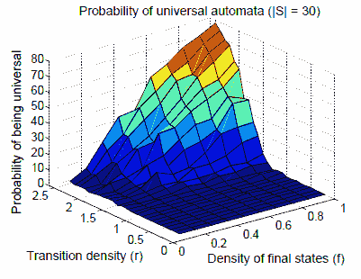
Fig. 1. Probability of universal automata (|S=30|)
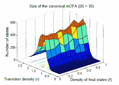
Fig. 2. Median number of state in the mDFA (|S=30|)
A completely different pattern emerges when we look at the size of canonical minimized DFA (mDFA) corresponding to the input NFA A (Figure 2). For each data point on the graph we determinized and minimized 200 random automata and took the median of the size of the minimized DFA (we chose to report the median rather than the mean because the median is less affected by outlying points). We refer to the latter as the canonical size. While the effect of the acceptance density on the canonical size is not too dramatic, transition density does have a dramatic effect on canonical size. The latter rises and then falls with tradition density, peaking at r = 1.25. We see that the canonical size has a coarse phase transition at that density.
Finally, we investigated how the canonical size scales with respect to the size of the input NFA A. Since the values of f do not have a large effect on the canonical size, we fixed f = 0.5 here. Figure 3 shows that canonical size scales differently at different transition densities. The scaling curves exhibit a range of behaviors. For r ≤ 1.25 they grow super–polynomially but subexponentially (in fact, a function of type ab√|S| provides a very good approximation), for r = 1.5 the growth is polynomial, and for higher transition densities they remain almost constant. Interestingly, though in the worst case the canonical size may scale exponentially [34], we do not observe such exponential scaling in our probabilistic model.
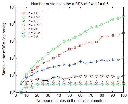
Fig. 3. Scaling of canonical size at different transition densities (log scale)
Based on these results we argue that our proposed model allows for “interesting” behavior as we vary r, f, and the size of the input NFA. In the next sections we use this model to study the performance of algorithms for canonization and universality.
3 Canonization
The canonization problem consists of constructing the minimal DFA that accepts the same language as a given (possibly non–deterministic) finite automaton. In addition to its theoretical appeal, this problem has an array of applications, from compilers to hardware circuit design to verification [40].
There are two different approaches to canonization. The first approach involves a two–step process: first, determinize the NFA, and second, minimize the resulting DFA. To complete the first step, we use the subset construction, which we present briefly here (see eg. [31] for a detailed description). Let A = (Σ, S, S0, ρ, F) be an NFA. We construct Ad = (Σ, 2S, {S0}, ρd, Fd), where Fd = {T ∈ 2S : T ∩ F 6=∅} and ρd(T1, a, T2) ⇐⇒ T2 = {t2 ∈ S : ρ(t1, a, t2) for some t1 ∈ T1}. The subset construction can be applied on the fly: starting with the initial state S0, we determine the “next” state for each letter, and then recur. The automaton Ad is deterministic and accepts exactly the same language as A. For the second step, Watson [40] presents 15 algorithms that can be used to minimize a DFA, including one of the simplest (Huffman’s [25]), and the one with the best known worst–case complexity (Hopcroft’s [23]). The second approach to canonization, due to Brzozowski [8], avoids the minimization step, but applies the determinization step twice. In our study we compare the two approaches by evaluating the performance of Hopcroft’s and Brzozowski’s algorithms on randomly generated automata.
We present briefly the idea of the two algorithms. Let L(A(p)) be the language accepted by the automaton A starting from the state p. Given a DFA, Huffman’s and Hopcroft’s algorithms construct an equivalence relation E ⊆ S × S with the following property: (p, q) ∈ E ⇔ L(A(p)) = L(A(q)). The equivalence relation E is computed as the greatest fixed point of the equation (p, q) ∈ E ⇔ (p ∈ F ⇔ q ∈ F)∧(∀a ∈ Σ, (p, a, p′) ∈ ρ, (q, a, q′) ∈ ρ : (p′, q′) ∈ E). In Huffman’s algorithm all states are assumed equivalent until proven otherwise.
Equivalence classes are split repeatedly until a fixpoint is reached. The algorithm runs in asymptotic time O(|S|2). Hopcroft made several clever optimizations in the way equivalence classes are split, which allowed him to achieve the lowest known running time O(|S|log|S|) [21, 23]. Hopcroft’s algorithm also significantly outperforms Huffman’s algorithm in practice, so we can ignore Huffman’s algorithm from this point on.
Strictly speaking, Hopcroft’s algorithm is just the DFA minimization algorithm, but we take it here to refer to the canonization algorithm, with determinization in the first step and minimization in the second step. Because the subset construction is applied in the first step, the worst–case complexity of this approach is exponential. Brzozowski’s algorithm is a direct canonization algorithm, and it does not use minimization, but, rather, two determinization steps. To describe the algorithm, we introduce some notation. If A is an automaton (Σ, S, S0, ρ, F), then reverse(A) is the automaton AR = (Σ, S, F, ρR, S0), where ρR ⊆ S ×Σ ×S and (s2, a, s1) ∈ ρR ⇔ (s1, a, s2) ∈ ρ. Intuitively, reverse switches the accepting and the initial states, and changes the direction of the transitions. Let determinize(A) be the deterministic automaton obtained from A using the subset construction, and let reachable(A) be the automaton A with all states not reachable from the initial states removed.
Theorem 1 (Brzozowski).
Let A be an NFA. Then A′ = [reachable ◦ determinize ◦ reverse]2(A) is the minimal DFA accepting the same language as A. It is not immediately obvious what the complexity of Brzozowski’s algorithm is.
The key to the correctness of the algorithm is, however, the following lemma.
Lemma 1.
Let A = (Σ, S, {s0}, ρ, F) be a DFA with the property that all states in S are reachable from s0. Then reachable(determinize(reverse(A))) is a minimal–state DFA.
Since the canonical size is at most exponential in the size of the input automaton and since reachable and determinize can be combined to generate only reachable sets (which is exactly what we do in Hopcroft’s algorithm), it follows that the worst–case complexity of Brzozowski’s algorithm is also exponential.
For our experimental study we used the tool dk.brics.automaton [32], developed by Anders Moller. All experiments were performed on the Rice Terascale Cluster3, which is a large Linux cluster of Itanium II processors with 4 GB of memory each. We first study performance on fixed–size automata. Again, our sample contains 200 random automata per (r, f) pair, and median time is reported (as we mentioned earlier, median time is less affected by outlying points than the mean. These, and all subsequent timing data, refer to the median). To generate each data point in Figure 4, we determinized and then minimized with Hopcroft’s algorithm each automaton; we measured combined running time for both steps. Note that Figure 4 is similar to Figure 2, but the two peaks occur in different densities (r = 1.5 and r = 1.25, respectively). As in Figure 2, for a fixed transition density, the impact of acceptance density on running time is not large.
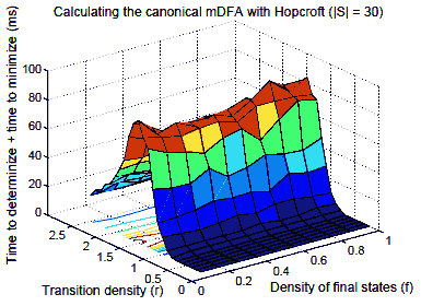
Fig. 4. Canonisation using Hopcroft
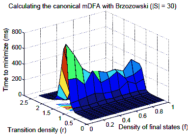
Fig. 5. Canonisation using Brzozowski
For Brzozowski’s algorithm,wemeasured the total time to performthe two reachable ◦ determinize ◦ reverse steps. The results are presented in Figure 5. The peak for Brzozowski’s algorithmcoincides with the peak of Figure 2 (r = 1.25). For a fixed transition density, the impact of acceptance density on running time is muchmore pronounced that in Hopcroft’s algorithm.
Our experiments indicate that neither Hopcroft’s nor Brzozowski’s algorithm dominates the other across the whole density landscape. In Figure 6 we show the running times of both algorithms for fixed f = 0.5. In Figure 6(a) the areas under both curves are 691 forHopcroft and 995.5 for Brzozowski, and in Figure 6(b) the areas are 1900 for Hopcroft and 5866 for Brzozowski, so Hopcroft’s algorithm has a better overall performance, but for r > 1.5 Brzozowski’s algorithm is consistently faster. The conclusion is that Hopcroft’s algorithm is faster for low–density automata, while Brzozowski’s algorithm is better for high–density automata. It remains to be seen if this conclusion applies also for automata that arise in practical applications, e.g, [1].
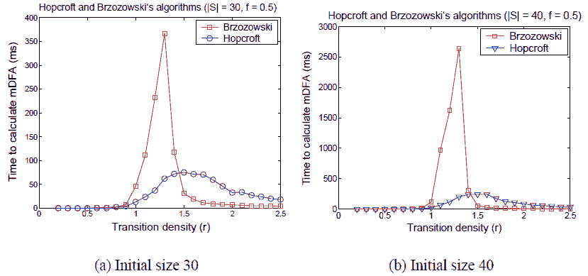
Fig. 6. Comparison between Hopcroft’s and Brzozowski’s algorithms for fixed f = 0.5
Similar to the approach of [36], we also investigated how Hopcroft’s and Brzozowski’s algorithms scale with automaton size. We fixed the acceptance density at f = 0.5, because its effect on the running time is less dramatic than that of the transition density.
The results (Figure 7) indicate that none of the algorithms scales better than the other over the whole landscape. Brzozowski’s algorithmhas an edge overHopcroft’s for r ≥ 1.5, and the opposite is true for the lower densities. At the peak, Hopcroft’s algorithm scales exponentially, but generally the algorithms scale subexponentially. Again we see that Hopcroft’s algorithm is better at low densities, while Brzozowski’s algorithm is better at high densities.
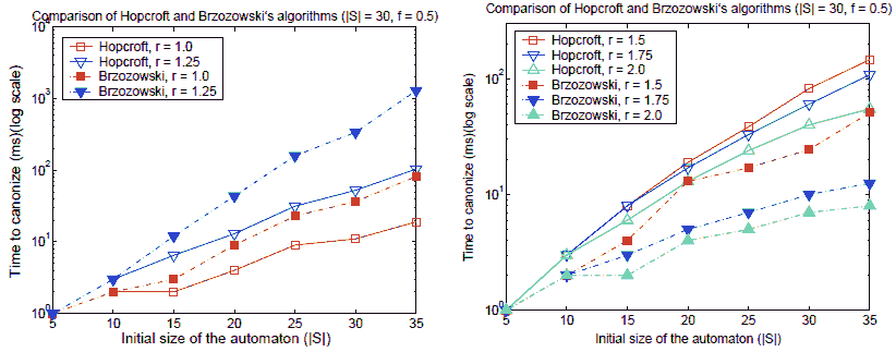
Fig. 7. Scaling comparison of Hopcroft and Brzozowski’s algorithms
4 Universality
The straightforward way to check for universality of an NFA A = (Σ, S, S0, ρ, F) is to determinize it, using the subset construction, and then verify that every reachable state is accepting and that the transition relation is total. We optimize this by modifying the subset construction algorithm slightly. When a “next” state is generated, the algorithm first checks whether it is accepting, and if this is not the case the algorithm terminates early, indicating that the automaton is not universal. An alternative approach is to view the determinized automatonAd = (Σ, 2S, {S0}, ρd, Fdwith Fd = {T ∈ 2S : T ∩ F 6= ∅} and ρd(T1, a, T2) ⇐⇒ T2 = {t2 ∈ S : ρ(t1, a, t2) for some t1 ∈ T1}, as a sequential circuit (SC). An SC [22] is a tuple (I,L, δ, α) where I is a set of input signals, L is a set of registers, δ : 2L × 2I → 2L is the next–state function, describing the next assignment of the of the registers given their current assignment and an input assignment, and α ∈ 2L is an initial assignment to the registers. (Usually we also have output signals and an output function, but this is not needed here.) The alphabet Σ = {0, 1} corresponds here to a single input signal. The state set S can be viewed as the register set L; a set in 2S can be viewed as a Boolean assignment to the state in S, using the duality between sets and their characteristic functions. The intuition is that every state in S can be viewed as a register that is either “active” or “inactive”. The initial state s0 correspond to an initial assignment, assigning 1 to s0 and 0 to all other registers, as only s0 is active, initially. Finally, the transition relation ρd, which is really a function, correspond to the next–state function, where δ(P, σ) = Q when ρd(P, a,Q) holds (note that we view here subsets of S as Boolean assignments to S). Universality of A now correspond to an invariance property of Ad, expressed in CTL as AG(Ws∈F s). Thus, we can check universality using a model checker.
In our evaluation we used two symbolic model checkers, both referred to as SMV: Cadence SMV [33] and NuSMV [15]. SMV is based on binary decision diagrams (BDDs) [8, 9], which provide a canonical representation for Boolean functions. A BDD is a rooted, directed acyclic graph with one or two terminal nodes labeled 0 or 1, and a set of variable nodes of out–degree two. The variables respect a given linear order on all paths from the root to a leaf. Each path represents an assignment to each of the variables on the path. Since there can be exponentially more paths than vertices and edges, BDDs are often substantially more compact explicit representations, and have been used successfully in the verification of complex circuits [12]. To encode the SC for Ad in SMV, we use the states in S as state variables, corresponding to the registers.
The SC is defined via the init and next statements: init(s) = 1 iff s = s0, and next(s) = 1 iff W_(t,_,s) t, when the input is σ; we provide an example in Figure 8.We use a Boolean array to encode the registers, and a variable input to encode the input symbol. The specification in the example is the universality property. The NFA A is universal iff the sequential circuit corresponding to Ad satisfies the specification. In order to improve the running time of the model checkers we considered several optimization techniques.
Sloppy vs. fussy encoding It turns out that to check universality we need not determinize A. Instead,we can construct the non–deterministic automat on An = (Σ, 2S, {S0}, ρn, Fd), with Fd = {T ∈ 2S : T ∩ F 6= ∅} and ρn(T1, a, T2) ⇐⇒ T2 ⊆ {t2 ∈ S : ρ(t1, a, t2) for some t1 ∈ T1}. It is easy to see that A is universal iff every reachable state in An is accepting. Intuitively, An allows more states to be active in the subset construction. Unlike Ad, we cannot view An as an SC, since it is not deterministic. SMV, however, can also model non–deterministic systems. Rather than require that next(s) = 1 iff W_(t,_,s) t, when the input is σ, we requite that next(s) = 1 if W_(t,_,s) t, when the input is σ (the “iff” is replaced by “if”). We refer to the initial encoding as fussy and to this encoding as sloppy. In an explicit construction the sloppy approach would generate more subsets, but in a symbolic approach the sloppy approach uses “looser” logical constraints (trans, rather than assign), which might result in smaller BDDs. See Figure 9 for a sloppy encoding of the previous example.
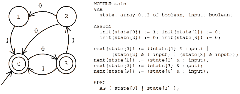
Fig. 8. A simple automaton and its encoding in SMV

Fig. 9. Sloppyencoding of the automaton in Figure 8
Monolithic vs. conjunctive partitioning In[11] Burch, Clarke and Long suggest an optimization of therepresentation of the transition relation of a sequential circuit.They note that the transition relation is the conjunction of severalsmall relations, and the size of the BDD representing the entiretransition relation may grow as the product of the sizes of theindividual parts. This encoding is called monolithic.The method that Burch et al. suggest represents the transition relation by a list of the parts, which areimplicitly conjuncted. Burch et al. call their method conjunctive partitioning,which has since then become the default encoding in NuSMV and CadenceSMV.
Conjunctive partitioning introduces an overhead when calculating the set ofstates reachable in the next step. The set of transitions has to beconsidered in some order, and choosing a good order is non–trivial,because each individual transition may depend on many variables. Inlarge systems the overhead is negligible compared to the advantage ofusing small BDDs [11]. However, in our models the transitions arefairly simple, and it is not immediately clear whether monolithicencoding is a better choice.
Variable ordering When using BDDs, it is crucial to select a good order of the variables.Finding an optimal order is itself a hard problem, so one has toresort to different heuristics. The default order in NuSMVcorresponds to the order in which the variables are first declared;in Cadence SMV it is based on some internal heuristic. The ordersthat we considered included the default order, and the orders givenby three heuristics that are studied with respect to treedecompositions: Maximum Cardinality Search (MCS), LEXP and LEXM [27].In our experiments MCS proved to be better than LEXP and LEXM, so wewill only report the results forMCS and the default order.
Inorder to apply MCS we view the automaton as a graph whose nodes arethe states, and in which two nodes are connected iff there is atransition between them. MCS orders [38] the vertices from 1 to |S|according to the following rule: The first node is chosen arbitrarily. Fromthis point on, a node that is adjacent to a maximal number of alreadyselected vertices is selected next, and so on. Ties can be broken invarious ways (eg. minimize the degree to unselected nodes [3] ormaximize it [5], or select one at random), but none leads to asignificant speedup. For our experiments, when we used MCS we broketies by minimizing the degree to the unselected nodes.
TraversalIn our model the safety condition is of the form AGα:i.e. α is a property that we want to hold in all reachable states. CTLformulas are normally evaluated backwards in NuSMV [16], via thegreatest fixpoint characterization: AGα= gfpZ[α ∧ AXZ]
Thisapproach (“backwards traversal”) can be sometimes quiteinefficient. As an optimization (only for AGαformulas), NuSMV supports another strategy: calculate the set ofreachable states, and verify that they satisfy the property α(“forward traversal”). In Cadence SMV, forward traversalis the default mode, but backwards traversal is also available. Weconsidered forward and backwards traversal for both tools.
Evaluating The Symbolic Approach Generally,running times of the various symbolic approaches increase with bothtransition density and acceptance density. In Figure 10 we presentthe effect of the first three optimizations (for this set ofexperiments forward traversal direction was used) to the runningtimes of NuSMV and Cadence SMV for fixed size automata. No singleconfiguration gives the best performance throughout the range oftransition density. Nevertheless, we can make several conclusionsabout the individual optimizations. Ordering the variables with MCSis always better than using the default ordering. Monolithic encodingis better than conjunctive partitioning for low transition density;the threshold varies depending on the tool and the choices for theother optimizations. Sloppy encoding is better than fussy when usedtogether with monolithic encoding; the opposite is true when usingconjunctive partitioning. The only exception to the latter is sloppymonolithic encoding in NuSMV, which gives the worst performance.Overall, for both tools, the best performance is achieved by usingmonolithic–MCS–sloppyupto r = 1.3, and conjunctive–MCS–⋆thereafter (the results for sloppy and fussy are too close to callhere).

Fig. 10. Optimizing the running times of NuSMV and Cadence SMV
In order to fine–tune the two tools we next looked at theirscaling performance (Figure 11). We considered automata with f = 0.9and r = 2.5 (our choice is explained later). We fixed the transitionencoding to conjunctive and variable order to MCS, and variedtraversal direction and sloppy vs. fussy encoding. For both toolsbackwards traversal is the better choice, not surprisingly, since 90%of the states are accepting and a fixed point is achieved veryquickly.When using backwards traversal, sloppy encoding gives betterperformance, and the opposite is true when using forward traversal.
Overall,the best scaling is achieved by Cadence SMV with backwards traversaland sloppy encoding, and this is what we used for comparison with theexplicit approach. ComparingThe Explicit and Symbolic Approaches Wecompared the performance of the explicit and the symbolic approacheson a set of randomautomata with a fixed initial size. For each datapoint we took the median of all execution times (200 sample points).Our results indicate that for small automata the explicit algorithmismuch faster than the symbolic. In fact, even when using automata withinitial size |S|=100, the median of the execution time is 0 almost everywhere on thelandscape (see Figure 12). In contrast, even for automata with |S|=30 the symbolic algorithm takes non–negligible time (Figure10).
As before, we also investigated which algorithm scales better as weincrease the initial size of the automata. For this set ofexperiments, we fixed the densities of the final states and thetransitions at f = 0.9 and r = 2.5 (i.e. on of the furthest edge ofthe landscape). We chose this point because almost everywhere elsethe median execution time of the explicit algorithm is 0 for smallautomata. We varied the initial size of the automata between 5 and600. The results are presented on Figure 13. The symbolic algorithm(Cadence SMV) is quite slower than the explicit throughout the wholerange. All algorithms scale sub–exponentially; however, thesymbolic algorithm scales
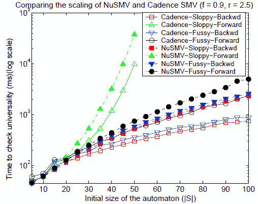
Fig. 11. OptimizingNuSMV and Cadence SMV (scaling)
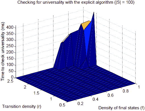
Fig. 12. Mediantime to check for universality with the explicit algorithm
2O(√|S|) worse than the explicit one (Figure 13(b)).We also present data forNuSMV, which scales the worst of the three algorithms and is the slowest for |S| >20.We note that at lower transition and/or acceptance density, theadvantage of the explicit approach over the symbolic approach is muchmore pronounced.
5 Discussion
In this paper we proposed a probabilistic benchmark for testingautomata–theoretic algorithms. We showed that in this modelHopcroft’s and Brzozowski’s canonization algorithms areincomparable, each having an advantage in a certain region of themodel. In contrast, the advantage of the explicit approach touniversality over the symbolic approach is quite clear.
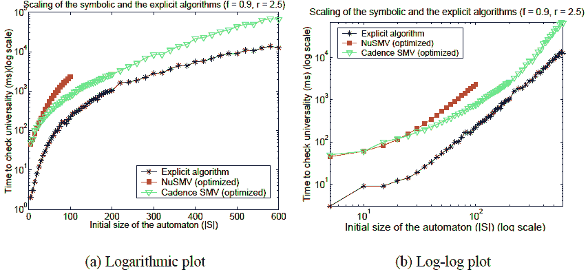
Fig. 13. Scalingcomparison of the symbolic and the explicit algorithms
An obvious question to raise is how “realistic” ourprobabilistic model is. There is no obvious answer to this question;partly because we lack realistic benchmarks of finite automata. Sinceautomata represent finite–state control, it is hard to see whyrandom directed graphs with linear density do not provide a realisticmodel. Hopefully, with the recent increase in popularity offinite–state formalisms in industrial temporal propertyspecification languages (c.f., [4, 6]), such benchmarks will becomeavailable in the not–too–far future, enabling us toevaluate our findings on such benchmarks. While our results arepurely empirical, as the lack of success with fully analyzing relatedprobabilistic models indicates (cf. [19, 18, 2]), providing rigorousproof for our qualitative observations may be a very challengingtask. At any rate, gaining a deeper understanding why one method isbetter than another method is an important challenge. Anotherresearch direction is to consider minimization on the fly, as, forexample, in [30].
Ourmost surprising result, we think, is the superiority of the explicitapproach to universality over the symbolic approach. This runsagainst the conventional wisdom in verification [12]. One may wonderwhether the reason for this is the fact that our sequential circuitscan be viewed as consisting of “pure control”, with nodata component, unlike typical hardware designs, which combinecontrol and data. This suggests that perhaps in model checking suchdesigns, control and data ought to be handled by differenttechniques. Another possible explanation is that the sequentialcircuits corresponding to the determinized NFA have registers withlarge fan–in, while realistic circuits typically havesmall–fan–in registers. We believe that these pointdeserve further study.
Infuture work we plan to extend the comparison between the explicit andsymbolic approaches to universality to automata on infinite words, aproblem of very direct relevance to computer–aided verification[29]. It is known that complementation of such automata is quiteintricate [29], challenging both explicit and symbolicimplementation.
Acknowledgments
.We are grateful to Andreas Podelski for raising the question ofcomparing Hopcroft’s and Brzozowski’s algorithms.
References
- Y. Abarbanel, I. Beer, L. Gluhovsky, S. Keidar, and Y. Wolfstal. FoCs – automatic generation of simulation checkers from formal specifications. In CAV, Proc. 12th International Conference, volume 1855 of LNCS, pages 538–542. Springer–Verlag, 2000.
- D. Achlioptas. Setting two variables at a time yields a new lower bound for random 3–SAT. In Proc. of 32nd Annual ACM Symposium on Theory of Computing, 2000.
- A. San Miguel Aguirre and M. Y. Vardi. Random 3–SAT and BDDs: The plot thickens further. In Principles and Practice of Constraint Programming, pages 121–136, 2001.
- R. Armoni, L. Fix, A. Flaisher, R. Gerth, B. Ginsburg, T. Kanza, A. Landver, S. Mador – Haim, E. Singerman, A. Tiemeyer, M.Y. Vardi, and Y. Zbar. The ForSpec temporal logic: A new temporal property–specification logic. In Proc. 8th International Conference on Tools and Algorithms for the Construction and Analysis of Systems, volume 2280 of LNCS, pages 296–211, Grenoble, France, April 2002. Springer–Verlag.
- D. Beatty and R. Bryant. Formally verifying a microprocessor using a simulation methodology. In Proc. 31st Design Automation Conference, pages 596–602. IEEE Computer Society, 1994.
- I. Beer, S. Ben–David, C. Eisner, D. Fisman, A. Gringauze, and Y. Rodeh. The temporal logic sugar. In Proc. 13th International Conference on Computer Aided Verification, volume 2102 of LNCS, pages 363–367, Paris, France, July 2001. Springer–Verlag.
- B. Bollobas. Random Graphs. Cambridge University Press, January 2001.
- R.E. Bryant. Graph–based algorithms for boolean–function manipulation. IEEE Trans. on Computers, C–35(8), 1986.
- R.E. Bryant. Symbolic boolean manipulation with ordered binary–decision diagrams. ACM Computing Surveys, 24(3):293–318, 1992.
- J.A. Brzozowski. Canonical regular expressions and minimal state graphs for definite events. In Mathematical theory of Automata, pages 529–561. Polytechnic Press, Polytechnic Institute of Brooklyn, N.Y., 1962. Volume 12 of MRI Symposia Series.
- J.R. Burch, E.M. Clarke, and D.E. Long. Symbolic model checking with partitioned transition relations. In Proc. IFIP TC10/WG 10.5 International Conference on Very Large Scale Integration, pages 49–58, 1991.
- J.R. Burch, E.M. Clarke, K.L. McMillan, D.L. Dill, and L.J. Hwang. Symbolic model checking: 1020 states and beyond. Information and Computation, 98(2):142–170, June 1992.
- Cadence. SMV. http://www.cadence.com/company/cadence labs research.html.
- P. Cheeseman, B. Kanefsky, andW. M. Taylor. Where the really hard problems are. In IJCAI ’91, pages 331–337, 1991.
- A. Cimatti, E. Clarke, E. Giunchiglia, F. Giunchiglia, M. Pistore, M. Roveri, R. Sebastiani, and A. Tacchella. NuSMV Version 2: An OpenSource Tool for Symbolic Model Checking. In Proc. International Conference on Computer–Aided Verification (CAV 2002), volume 2404 of LNCS, Copenhagen, Denmark, July 2002. Springer.
- A. Cimatti, E. M. Clarke, F. Giunchiglia, and M. Roveri. NUSMV: A new symbolic model checker. International Journal on Software Tools for Technology Transfer, 2(4):410–425, 2000.
- E.M. Clarke, O. Grumberg, and D. Peled. Model Checking. MIT Press, 1999.
- Olivier Dubois, Yacine Boufkhad, and Jacques Mandler. Typical random 3–SAT formulae and the satisfiability threshold. In SODA, pages 126–127, 2000.
- E. Friedgut. Necessary and sufficient conditions for sharp thresholds of graph properties, and the k–SAT problem. Journal of the A.M.S., 12:1017–1054, 1999.
- James Glenn and William I. Gasarch. Implementing WS1S via finite automata: Performance issues. In Workshop on Implementing Automata, pages 75–86, 1997.
- D.Gries. Describing an algorithm by Hopcroft. Acta Informatica, 2:97–109, 1973.
- G.D. Hachtel and F. Somenzi. Logic Synthesis and Verification Algorithms. Kluwer Academic Publishers, Norwell, Massachusetts, 1996.
- J.E. Hopcroft. An n log n algorithm for minimizing the states in a finite automaton. In Z. Kohavi, editor, The Theory of Machines and Computations, pages 189–196. Academic Press, 1971.
- J.E. Hopcroft and J.D. Ullman. Introduction to Automata Theory, Languages, and Computation. Addison–Wesley, 1979.
- D.A. Huffman. The synthesis of sequential switching circuits. In E. F. Moore, editor, Sequential Machines: Selected Papers. Addison–Wesley, 1964.
- R.M. Karp. The transitive closure of a random digraph. Random Struct. Algorithms, 1(1):73– 94, 1990.
- C.A. Koster, H. L. Bodlaender, and C. P. M. van Hoesel. Treewidth: Computational experiments. ZIB–Report 01–38, Konrad–Zuse–Zentrum f.ur Informationstechnik Berlin, Berlin, Germany, 2001. Also available as technical report UU–CS–2001–49 (Utrecht University) and research memorandum 02/001 (Universiteit Maastricht).
- O. Kupferman and M.Y. Vardi. Model checking of safety properties. Formal methods in System Design, 19(3):291–314, November 2001.
- O. Kupferman and M.Y. Vardi. Weak alternating automata are not that weak. ACM Trans. on Computational Logic, 2001(2):408–429, July 2001.
- D. Lee and M. Yannakakis. Online minimization of transition systems. In Proc. 24th ACM Symp. on Theory of Computing, pages 264–274, Victoria, May 1992.
- P. Linz. An introduction to formal languages and automata. D. C. Heath and Company, Lexington, MA, USA, 1990.
- A. Moller. dk.brics.automaton. http://www.brics.dk/automaton/, 2004.
- K.L. McMillan. Symbolic Model Checking. Kluwer Academic Publishers, 1993.
- A.R. Meyer and M.J. Fischer. Economy of description by automata, grammars, and formal systems. In Proc. 12th IEEE Symp. on Switching and Automata Theory, pages 188–191, 1971.
- A.R. Meyer and L.J. Stockmeyer. The equivalence problem for regular expressions with squaring requires exponential time. In Proc. 13th IEEE Symp. on Switching and Automata Theory, pages 125–129, 1972.
- G. Pan and M.Y. Vardi. Search vs. symbolic techniques in satisfiability solving. In SAT 2004, LNCS, Aalborg, May 2004. Springer–Verlag.
- Bart Selman, David G. Mitchell, and Hector J. Levesque. Generating hard satisfiability problems. Artificial Intelligence, 81(1–2):17–29, 1996.
- R.E. Tarjan and M. Yannakakis. Simple linear–time algorithms to test chordality of graphs, test acyclicity of hypergraphs, and selectively reduce acyclic hypergraphs. SIAM J. Comput., 13(3):566–579, 1984.
- M.Y. Vardi and P. Wolper. An automata–theoretic approach to automatic program verification. In Proc. 1st Symp. on Logic in Computer Science, pages 332–344, Cambridge, June 1986.
- B.W. Watson. A taxonomy of finite automata minimization algorithmes. Computing Science Note 93/44, Eindhoven University of Technology, The Netherlands, 1993.
- B.W. Watson. Taxonomies and Toolkits of Regular Language Algorithms. PhD thesis, Eindhoven University of Technology, the Netherlands, 1995.