
Abstract
Research of a fan electric drive with permanent magnet synchronous machine
Content
- Introduction
- 1. Theme urgency
- 2. Constructions and types of PMSM
- 3. Control algorithms
- 3.1 Hall sensor control
- 3.2 Sensorless control for direct measurement of the back EMF
- 3.3 Sensorless control for the indirect measurement of the back EMF
- 4. Choice of hardware
- 4.1. Power section
- 4.2 Target platform
- Conclusion
- References
Introduction
This article is devoted to the development and expediency of the ESC control algorithm modernization for PMSM with trapezoidal form of back-EMF applied as traction electric drive of the propeller motor group. Analysis and selection of the optimal control algorithm for various criteria (thrust / current, quality of regulation / cost, etc.).
1. Theme urgency
The electric drive with a fan characteristic is the most common and is found almost everywhere. Even your home probably has such a mechanism (a cooler in a PC, air conditioners, vacuum cleaners). In the general case, for these mechanisms, absolutely all types of electric motors are suitable, however, the use of a synchronous motor with permanent magnets is of the greatest interest, this statement is due to the fact that:
- PMSM have the highest efficiency (about 2% more than the highly efficient (IE3) asynchronous motor [ 1 ])
- Have the best, among all types of electric motors, power / weight, torque / inertia, etc.
- It has a lower speed control range than the AD, which corresponds to the requirements of the mechanism with a fan-like nature of the load.
With the development of semiconductor and microprocessor technology, it became possible to use PMSM as a regulated electric drive (with a range of regulation from zero to speed-limited motor speed specifications, even for sensorless systems), which greatly expanded the area of application up to aircraft modeling, robotics, and machine building.
When using PMSM as a drive for a propeller-driven group, in particular for aircraft modeling, the issue of operating time from the battery that can be solved by developing a control system that would allow maximum traction with a minimum of current consumption is acute. Also, the control system must have robustness. The motor is constantly affected by various kinds of disturbances (gusts, vibrations from neighboring motors, etc.).
2. Constructions and types of PMSM
2.1. According to the location of the rotor
The rotor can be located inside the stator (Inrunner) or outside (Outrunner) . motors with an external rotor, as a rule, have a smaller inertia.
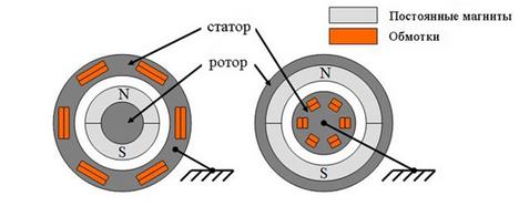
Figure 1 – PMSM classification of the rotor location
2.2. According to the design of the rotor
- Motors with pronounced poles
- Electric motors with implicitly expressed poles
The motor with implicitly expressed poles has equal inductance along the longitudinal and transverse axes Ld = Lq, whereas in the case of a motor with pronounced poles the transverse inductance is not equal to the longitudinal inductance Lq! = Ld [ 2 ].
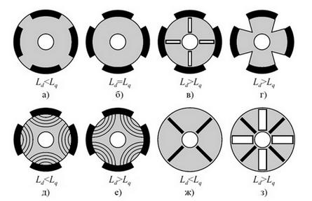
Figure 2 – Cross section of rotors with different Ld / Lq ratio. Black designates magnets. Figure d , e are presented axially stratified rotors in the figure in and z are shown rotors hurdles.
2.3 By location of magnets
- Synchronous motor with surface permanent magnet synchronous motor ( SPMSM )
- Synchronous motor with integrated magnets ( IPMSM – interior permanent magnet synchronous motor )
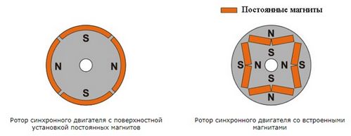
Figure 3 – Classification of PMSM in the arrangement of magnets
2.4. The stator construction
Depending on the stator design, a synchronous motor with permanent magnets can be:
- With distributed winding
- With concentrated winding
Distributed is called a winding, in which the number of slots per pole and phase Q = 2,3, ..., k. Concentrated is called a winding, in which the number of slots per pole and phase Q = 1. In this case, the grooves are arranged evenly along the circumference of the stator. The two coils forming the winding can be connected either in series or in parallel. The main drawback of such windings is the impossibility of influencing the shape of the emf curve [ 2 ].
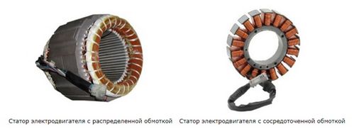
Figure 4 – External differences of concentrated and distributed windings PMSM
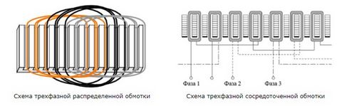
Figure 5 – Schematic differences between concentrated and distributed windings PMSM
2.5. In the form of a back emf
The form of the back-EMF of the electric motor can be:
- Trapezoidal
- Sinusoidal
The shape of the EMF curve in the conductor is determined by the distribution curve of the magnetic induction in the gap along the circumference of the stator. It is known that the magnetic induction in the gap under the pronounced pole of the rotor has a trapezoidal shape. The same form has the EMF induced in the conductor. If it is necessary to create a sinusoidal emf, the pole pieces are shaped in such a way that the induction curve is close to sinusoidal. This is facilitated by the bevels of the pole pieces of the rotor [ 3 ].
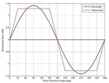
Figure 6 – Differences in the form of the back-EMF of PMSM
3. Control algorithms
As the considered motor is adopted PMSM type OUTRUNNER , with pronounced poles, surface installation of magnets, distributed winding and trapezoidal form of back-EMF. Such motors are sometimes referred to as DC brushless electric motors (BLDC) .
The control algorithms of the BLDC / PMSM with trapezoidal feedback emf can be divided into:
- Control without feedback (relevant only for applications where the load is known in advance and does not change during operation and low reliability requirements)
- Control using rotor position sensors (Hall sensors, encoders, tachogenerators, etc.)
- Sensorless control, in which to identify the position of the rotor is used:
- Measurement of the back-emf in one phase
- Analysis of the response to the HF signal for the motors with Lq! = Ld (HFI method)
You can neglect the form of the back-EMF of the motor and apply control algorithms for the PMSM with a sinusoidal back-EMF (scalar(V/F), FOC, DTC) while the torque pulsations can reach 17% [ 2 ].
Sensorless control, depending on the method of measuring the back-emf can be divided into:
- Direct measurement of the back EMF (determining the moment of transition of the EMF through 0 for which the voltage of the midpoint is taken.Due to the use of PWM are required voltage dividers and low-pass filters)
- Indirect measuring the back EMF (Since the signal filtering in the direct measurement of the delay introduced at high speed and bandpass filter leads to signal attenuation at low speed used indirect methods of determining back emf)
- Integration of back emf
- Integration of the 3rd harmonic of the voltage
When using PMSM with trapezoidal back-emf as a drive of a propeller-driven group, it is recommended to use only sensorless control algorithms. the presence of sensors significantly reduces the reliability of the system due to severe operating conditions (vibration, high dynamic loads, high humidity and a large amount of dirt and dust), which is unacceptable. However, the control algorithm for Hall sensors is the most obvious for understanding the physical principles of PMSM management and will also be considered as an example.
One of the drawbacks of the sensorless control of PMSM is the problem of starting and running at low speed when the amplitude of the back EMF is comparable to the amplitude of the noise from the sensors. It is worth noting that for mechanisms with fan load this problem is not critical because there is no need to develop a high torque at zero and low revs. To solve this problem, use the following methods:
- Sensorless start:
- Initial alignment of the rotor by specifying a fixed current vector of the safe amplitude
- Waiting for the positioning of the rotor in accordance with the stator current vector
- Acceleration without feedback until the moment when the magnitude of the back-EMF becomes sufficient to determine the position of the rotor
- Determination of the initial rotor position in the stopped state:
- Short pulses are alternately applied to each of the phases.
- The response to each of the pulses relative to the midpoint
- The difference in response determines the initial position of the rotor
3.1 Hall sensor control
For estimating the rotor position, three hall sensors are positioned. These hall sensors are separated by 120° each. With these sensors, 6 different commutations are possible. Phase commutation depends on hall sensor values. Power supply to the coils change when hall sensor values change. With right synchronized commutations, the torque remain nearly constant and high.
To simplify the explanation of how to operate a three phases BLDC motor a typical BLDC motor with only three coils is considered. As previously shown, phases commutation depends on the hall sensor values. When motor coils are correctly supplied, a magnetic field is created and rotor moves. The most elementary commutation driving method used for BLDC motors is an on-off scheme: a coil is either conducting or not conducting. Only two windings are supplied at the same time the third winding is floating. Connecting the coils to the power and neutral bus induces the current flow. This is referred to as trapezoidal commutation or block commutation. [ 5 ].
To control the BLDC, a power cascade consisting of 3 half-bridges is used. The power stage diagram is shown in Figure 7
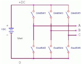
Figure 7 – Power stage
Based on the readings of Hall sensors, it is determined which keys should be closed.
Table 1 – Switching the keys clockwise.
| Value of Hall sensors (Hall_CBA) | Phase | Keys |
|---|---|---|
| 101 | A-B | SW1, SW4 |
| 001 | A-C | SW1, SW6 |
| 011 | B-C | SW3, SW6 |
| 010 | B-A | SW3, SW2 |
| 110 | C-A | SW5, SW2 |
| 100 | C-B | SW1, SW4 |
The strength of the magnetic field determines the force and speed of the motor. By varying the current flow through the coils the speed and torque of the motor can be adjusted. The most common way to control the current flow is to control the average current flow through the coils. PWM(Pulse Width Modulation) is used to adjust the average voltage and thereby the average current, including the speed. The speed can be adjusted with a high frequency from 20 khz to 60 khz. The rotating field of a three-phase, three-winding BLDC is shown in Figure 8
Figure 8 – Switching steps and rotating field
(animation: 6 frames, 10 cycles, 63.7 kilobytes)
Commutation creates a rotating field. Step1 Phase A is connected to the positive DC bus voltage by SW1 and Phase B is connected to ground
by SW4, Phase C is unpowered. Two flux vectors are generated by phase A (red arrow) and phase B (blue arrow) the sum of the two vectors give
the stator flux vector (green arrow). Then the rotor tries to follow stator flux. As soon as the rotor reach a certain position when the hall
sensors state changes its value from 010
to 011
a new voltage pattern is selected and applied to the BLDC motor.
Then Phase B is unpowered and Phase C is connected to the ground. It results in a new stator flux vector (Step2). If we follow the switching
scheme shown in figure 8 and in Table 1, we obtain six different magnetic flux vectors corresponding to six switching stages.
Six stages correspond to one revolution of the rotor. [ 5 ]
3.2 Direct Emf Measurement
The overwhelming majority of controllers (ESC) for drives of the propeller motor group work according to the algorithm given below or use another without fundamental differences.
The typical trapezoidal back-EMF waveforms and corresponding driving voltages of a 3-phase BLDC are shown in Figure 9. In every commutation step,
one phase winding is connected to positive supply voltage, one phase winding is connected to negative supply voltage and one phase is floating.
The back-EMF in the floating phase will result in a zero crossing when it crosses the average of the positive and negative supply voltage.
The zero crossings are marked as ZC(ПН
) in Figure 9. The intersection of zero always arises at the center between two commutations. At a constant
speed or a slowly varying speed, the time from one commutation to the intersection of zero and the time from zero
to the next commutation are equal. This is used as a basis in this implementation of the control device without the use of sensors.
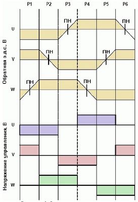
Figure 9 – Oscillograms of signals
The motor speed/torque is controlled by pulse width modulation (PWM). It is important to understand how the PWM works and how it interacts with the analog to digital converter (ADC) in order to make reliable measurements in the noisy environment created by the PWM. The PWM is used in what is called phase correct mode. This mode uses a counter in a dual slope operation that makes the PWM output symmetrical within one PWM period. Furthermore, the compare value that determines the duty cycle of the PWM output is buffered, so it is not updated in the middle of a PWM cycle. Figure 10 shows the relationship between counter value, compare value and PWM output. Each PWM period is separated by dashed lines in the figure. The figure also shows that an overflow event occurs when the timer reaches zero. This event can be used to automatically trigger an ADC sample. Unless the duty cycle is very low, this is a point where the PWM output has been stable for a long time. This is used to make sure that the ADC sample of the floating phase voltage is made when the PWM switching noise is low.
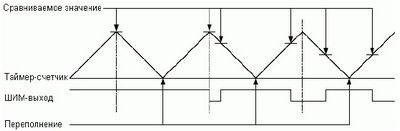
Figure 10 – PWM generation
The zero-crossing happens when the floating phase crosses the average voltage of the two supply rails. In this application note, it is assumed that the negative supply is at ground level, which makes the zero-cross voltage half the motor supply voltage. This dependence on motor supply voltage makes it impractical to use a fixed zero cross voltage threshold. Instead, the motor supply voltage (or scaled down version) is used as ADC reference voltage. The motor supply voltage needs to be low pass filtered before it is fed to the ADC. The VD/LPF should be used for this purpose. The DC gain should be selected so that the voltage will be in the allowable range for the ADC, between 1.0V and AVCC. The three phase voltages should be connected to the ADC through 3 VD/LPFs. The filters should have the same DC gain as the ADC reference in order to utilize the full ADC voltage range. The low pass filter should be designed to filter out as much high frequency noise as possible without introducing notable delay to the back-EMF signal.
3.3 Indirect measurement back emf
Since the scheme of direct measurement of the back-EMF has a number of drawbacks:
- Filtering the signal with direct measurement introduces delay at high speed and the filter bandwidth results in signal attenuation at low speed.
- Switching moments can
float
in dynamic modes (acceleration / deceleration)
The scheme of indirect EMF measurement based on the integration of back-EMF will be considered. The algorithm for the indirect determination of the back-EMF differs from the direct only in the software implementation and does not affect the circuitry in any way (it is identical to that described in 3.2.) In the direct method of measuring the emf, the moment of the transition through 0 is determined after a timing that depends on the current speed and inductance (at high speed, the switching neEMF to be done earlier so that the current can reach the maximum value at the right time) after the inverter passes to the next state. The main problem of this method is that, due to the above disadvantages, the time delay depends on the speed and is subject to the influence of noise.
Indirect way works as follows:
- The instant of transition through 0 is determined as in the direct method.
- Instead of time delay, the microcontroller ADC starts to make samples at fixed intervals and summarize the results.
- When the sum of the ADC samples becomes equal to or greater than the user-selected setpoint, the integrator is reset and the inverter is switched to the next state.
The main advantage of this method is a lower sensitivity to noise and adaptation to the change in speed. This statement is based on the fact that the area under the line between the points of intersection of zero and the setpoint of the trip (forms the shape of a triangle) does not change during acceleration / deceleration, does not depend on speed and delay, in electric degrees, between the determination of the transition through 0 and the transition to the next state Inverter is always constant. Because at low rotor speed the EMF value is small and the integrator accumulates the required value longer and on high EMF higher and accordingly the integrator reaches the setpoint value earlier.
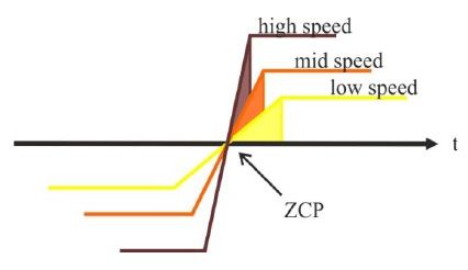
Figure 11 – Sites of integration of back-emf
4. Hardware Description
4.1. Power section
A typical block diagram of the device is shown in Figure 4.1 and includes the following elements:
- Inverter (three-phase bridge circuit on N-channel MOS transistors)
- Inverter driver
- Back EMF sensors (phase-to-phase voltage dividers and low-pass filters)
- Current sensors
- DC link voltage sensor
- Microcontroller power supply
- Microcontroller
Also, in the device, without fail, there must be a communication interface, debug outputs. Each structural element has an appropriate switching circuit, the complete circuit diagram of the device is presented in the thesis.
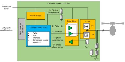
Figure 12 – Block diagram of the controller
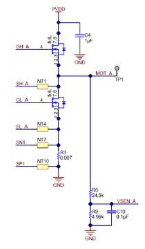
Figure 13 – Inverter rack layout
4.2 Target platform
As the control device for the controller (ESC), the microcontroller STM32F103 was selected whose brief technical characteristics are presented in Table 2.
Table 2 – Characteristics of the selected microcontroller.
| Parameter | Value |
|---|---|
| core | ARM Cortex M3 |
| clock frequency | up to 72MHz |
| FLASH memory | 32 ... 128kb |
| SRAM-memory | up to 20kb |
| interfaces | SPI, I2C, USART, USB 2.0, CAN |
| ADC | up to two 12 bits / 16 channels |
| timers | 7, including 1 motor control |
| consumption current | up to 2 uA in standby mode |
| temperature Range | -40 ° C ... 125 ° C |
| types of housings | VFQFPN36, LQFP48, LQFP64, LQFP100 |
| supply voltage | 2 ... 3.6V |
This microcontroller has been selected as the target platform due to the following advantages:
- Availability of a fast, flexibly adjustable, motor control timer that has 4 comparator / PWM channels with complementary pairs and the possibility of hardware generation of dead time between them. Rationale: For the ESC motors used, a high PWM frequency (greater than 20 KHz) is required to maintain the continuous current mode because they have a very small electromagnetic time constant.
- Two fast (1.15 microseconds with 72 MHz clock), 12-bit ADCs with the ability to simultaneously sample on several channels. Justification: To reduce the influence of noise, sampling ADCs from different sensors of the same type must be done simultaneously.
- Sufficient performance for implementing complex control algorithms. Rationale: It is necessary to provide the possibility of implementing the field of an oriented control algorithm in a sensorless mode.
- Variety of communication interfaces. Justification: Different flight controllers can send a control signal to the ESC via different protocols.
- Low price (comparable with 8-bit microcontrollers).
Conclusion
The controllers (ESC) used in the mass production of drives of propeller-driven groups use the motor control algorithms, which are not optimal from the point of view of the produced thrust per unit of current consumed and, consequently, from the point of view of energy efficiency. Moreover, high torque and thrust pulsations supplemented by external disturbances can lead to loss of stability, unnecessary vibrations and will significantly complicate the task of stabilizing the multi-rotor system. The application of algorithms for the indirect determination of the back-emf or the field-oriented control algorithm will eliminate the above described shortcomings or significantly reduce their effect on the system.
References
- Markus Lindegger. Economic viability, applications and limits of efficient permanent magnet motors. Switzerland: Swiss Federal Office of Energy, 2009
- Design and Prototyping Methods for Brushless Motors and Motor Control.-MIT, 2010
- Synchronous motors with permanent magnets.
Access mode: motorering companymotorering solutions
- Calculator tyagovoruzhennosti multi-rotor systems
Access mode: Internet resourceeCalc
- AVR492: DC brushless motor control with AT90PWM3.- Atmel
- AVR444: Control of a three-phase brushless DC motor without sensors. – Atmel
- STM32F103 Datasheet: DocID13587 Rev 17.- ST Microelectronics, 2015
- STM32F103 Reference manual: DocID13902 Rev 16.- ST Microelectronics, 2015
- Position and Speed Control of Brushless DC Motors Using Sensorless Techniques and Application Trends.- Department of Signal Theory, Communications and Telematic motorering, University of Valladolid (UVA), 47011 Valladolid, Spain, 2010
- Sensorless Detection of Rotor Position of PMBL Motor at Stand Still / Roustiam Chakirov, Yuriy Vagapov, and Andreas Gaede / WCECS 2007, October 24-26, 2007, San Francisco, USA