Implementation of Training Convolutional
Neural Networks
Tianyi Liu, Shuangsang Fang, Yuehui Zhao, Peng Wang, Jun Zhang
University of Chinese Academy of Sciences, Beijing, China
{liutianyi14@mails.ucas.ac.cn}
ABSTRACT
Deep learning refers to the shining branch of machine learning that is based on learning
levels of representations. Convolutional Neural Networks (CNN) is one kind of deep neural
network. It can study concurrently. In this article, we gave a detailed analysis of the process of
CNN algorithm both the forward process and back propagation. Then we applied the particular
convolutional neural network to implement the typical face recognition problem by java. Then, a
parallel strategy was proposed in section4. In addition, by measuring the actual time of forward
and backward computing, we analysed the maximal speed up and parallel efficiency theoretically.
Keywords: Convolutional Neural Networks, face training, Parallel Strategy, Maximal speedup
1. INTRODUTION
Deep learning refers to a subfield of machine learning that is based on learning levels of
representations, corresponding to a hierarchy of features, factors or concepts, where higher-lever
concepts are defined from lower-lever ones, and the same lower-lever concepts can help to define
many higher-lever concepts.
Deep learning is learning multiple levels of representation and abstraction, helps to
understand the data such as images, audio and text. The concept of Deep Learning comes from the
study of Artificial Neural Network, Multilayer Perceptron which contains more hidden layers is a
Deep Learning structure.
In the late 1980s, the invention of Back Propagation algorithm used in Artificial Neural
Network brings hope to machine learning and creates a trend of machine learning based on
statistical models. In the 1990s, a variety of Shallow Learning models have been proposed such as
Support Vector Machines (SVM), Boosting, Logistic Regression (LR). The structure of these
models can be seen as one hidden node (SVM, Boosting), or no hidden nodes (LR). These models
gained a great success both in theoretical analysis and applications.
In 2006, Geoffrey Hinton who is the professor of University of Toronto, Canada and the dean
of machine learning and his students Ruslan Salakhutdinov published an article in “Science”, led
to a trend of machine learning in academia and industry. The article had two points: 1) Artificial
Neural Network with multiple hidden layers has an excellent ability of characteristic learning. The
characteristics obtained from learning have an essential description to data, then facilitate
visualization or classification. 2) The difficulties of deep neural network in training can overcome
by layer-wise pre-training. In this article, the implementation of layer-wise pre-training is
achieved through unsupervised learning.
Feedforward neural network or Multilayer Perceptron with multiple hidden layers in artificial
neural networks is usually known as Deep Neural Networks (DNNs). Convolutional Neural
Networks (CNN) is one kind of feedforward neural network. In 1960s, when Hubel and Wiesel
researched the neurons used for local sensitive orientation-selective in the cat’s visual system, they
found the special network structure can effectively reduce the complexity of Feedback Neural
Networks and then proposed Convolution Neural Network. CNN is an efficient recognition
algorithm which is widely used in pattern recognition and image processing. It has many features
such as simple structure, less training parameters and adaptability. It has become a hot topic in
voice analysis and image recognition. Its weight shared network structure make it more similar to
biological neural networks. It reduces the complexity of the network model and the number of
weights.
Generally, the structure of CNN includes two layers one is feature extraction layer, the input
of each neuron is connected to the local receptive fields of the previous layer, and extracts the
local feature. Once the local features is extracted, the positional relationship between it and other
features also will be determined. The other is feature map layer, each computing layer of the
network is composed of a plurality of feature map. Every feature map is a plane, the weight of the
neurons in the plane are equal. The structure of feature map uses the sigmoid function as
activation function of the convolution network, which makes the feature map have shift invariance.
Besides, since the neurons in the same mapping plane share weight, the number of free parameters
of the network is reduced. Each convolution layer in the convolution neural network is followed
by a computing layer which is used to calculate the local average and the second extract, this
unique two feature extraction structure reduces the resolution.
CNN is mainly used to identify displacement, zoom and other forms of distorting invariance
of two-dimensional graphics. Since the feature detection layer of CNN learns by training data, it
avoids explicit feature extraction and implicitly learns from the training data when we use CNN.
Furthermore, the neurons in the same feature map plane have the identical weight, so the network
can study concurrently. This is a major advantage of the convolution network with respect to the
neuronal network connected to each other. Because of the special structure of the CNN’s local
shared weights makes it have a unique advantage in speech recognition and image processing. Its
layout is closer to the actual biological neural network. Shared weights reduces the complexity of
the network. In particular multi-dimensional input vector image can directly enter the network,
which avoids the complexity of data reconstruction in feature extraction and classification process.
Face recognition is a biometric identification technology based on the facial features of
persons. The study of face recognition system began in the 1960s, in the late 1980s with the
development of computer technology and optical imaging techniques it has been improved; in the
late
1990s it truly entered the stages of initial applications. In practical applications, such as
monitoring system, the collected face images captured by cameras are often low resolution and
with great pose variations. Affected by pose variation and low resolution, the performance of face
recognition degrades sharply. And pose variations bring great challenge to face recognition. They
bring nonlinear factors into face recognition. And some of the existing machine learning method
mostly use shallow structure. Deep learning can achieve the approximation of complex function
by a deep nonlinear network structure.
In this article, we use convolution neural network to solve face recognition. It can overcome
the influence of pose or resolution in face recognition. Due to the long training time and the large
recognition computing, it is difficult to meet the real-time requirements, or the delay exceeds the
range of tolerance. So we use the cloud platform to concurrently speed up the computing process.
2. BACKGROUND AND RELATED WORK
Convolutional Neural Networks can be applied in many different areas. Yann LeCun and his
team specially designed Convoutional Neural Networks to deal with the variability of 2D shapes,
which are shown to outperform all other techniques.[1] Dan C and his team present a fast, fully
parameterizable GPU implementation of Convolutional Neural Network variants for Image
Classification. [2] Another team proposes two novel frontends for robust language identification
(LID) using a convolutional neural network (CNN) trained for automatic speech recognition
(ASR). [5] What’s more, Convolutional Neural Networks are used in Visual Recognition[9] and
many other areas, such as Facial Point Detection[6], House Numbers Digit Classification[10],
Multi-digit Number Recognition from Street View Imagery[11].
Besides these works, many teams are focusing on the speed up of ConvNets. For example,
Multi-GPU Training of ConvNets. In this work
, Facebook AI Group consider a standard
architecture [1] trained on the Imagenet dataset [2] for classification and investigate methods to
speed convergence by parallelizing training across multiple GPUs.[4]
3. PRINCIPLE OF CONVELUTIONAL NEURAL NETWORKS
3.1 Methodology
Convolution neural network algorithm is a multilayer perceptron that is the special design for
identification of two-dimensional image information
. Always has more layers: input layer,
convolution layer, sample layer and output layer. In addition, in a deep network architecturethe
convolution layer and sample layer can have multiple. CNN is not as restricted boltzmann
machine, need to be before and after the layer of neurons in the adjacent layer for all connections,
convolution neural network algorithms, each neuron don't need to do feel global image, just feel
the local area of the image. In addition, each neuron parameter is set to the same, namely, the
sharing of weights , namely each neuron with the same convolution kernels to deconvolution
image.
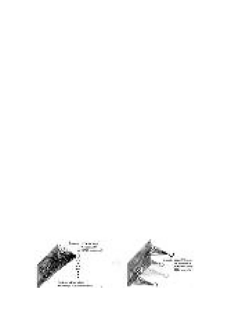
Fig 1 fully connection vs partial connection
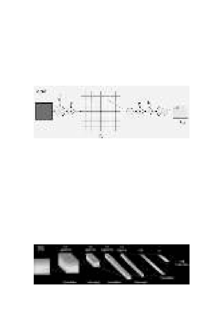
CNN algorithm has two main processes: convolution and sampling .
Convolution process: use a trainable filter Fx, deconvolution of the input image
(the first stage is the input image, the input of the after convolution is the feature
image of each layer, namely Feature Map), then add a bias bx, we can get convolution
layer Cx.
A sampling process: n pixels of each neighborhood through pooling steps,
become a pixel, and then by scalar weighting Wx + 1 weighted, add bias bx + 1, and
then by an activation function, produce a narrow n times feature map Sx + 1.
Fig 2 main process of CNN
The key technology of CNN is the local receptive field, sharing of weights ,
sub sampling by time or space, so as to extract feature and reduce the size of the
training parameters.The advantage of CNN algorithm is that to avoid the explicit
feature extraction, and implicitly to learn from the training data;The same neuron
weights on the surface of the feature mapping, thus network can learn parallelly ,
reduce the complexity of the network;Adopting sub sampling structure by time or
space, can achieve some degree of robustness, scale and deformation
displacement;Input information and network topology can be a very good match, It
has unique advantages in speech recognition and image processing.
3.2 CNN Architecture Design
CNN algorithm need experience in architecture design, and need to debug unceasingly in the
practical application, in order to obtain the most suitable for a particular application architecture of
CNN. Based on gray image as the input of 96
96, in the preprocess stage, turning it into 32
32 of the size of the image. Design depth of the layer 7 convolution model: input layer,
convolution layer C1, sub sampling layer S1, convolution layer C2, sampling layer S2, hidden
layer H and output layer F.
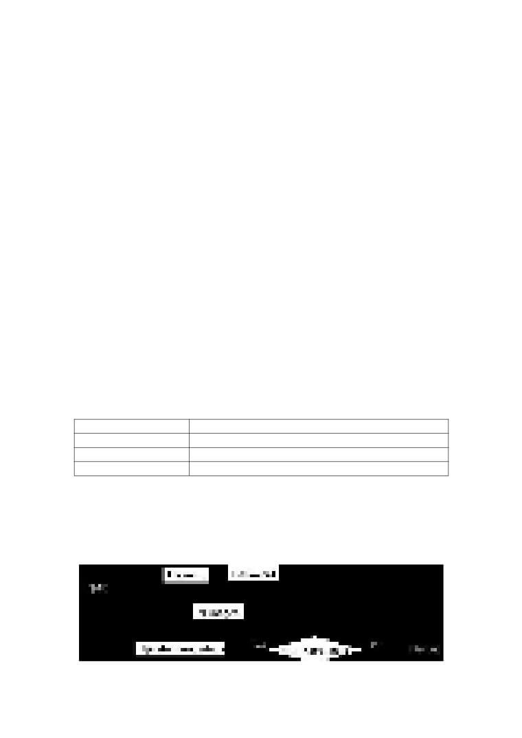
Fig 3 architecture of CNN in training faces
In view of the 32
32 input after preprocessing, There is a total of 17 different pictures.
C1 layer for convolution, convolution layer adopts 6 convolution kernels, each the size of the
convolution kernels is 5
5, can produce six feature map, each feature map contains (32-5 + 1)
(32-5 + 1) = 28
28 = 784 neurons. At this point, a total of 6
(5
5 + 1) = 156
parameters to be trained .
S1 layer for sub sampling, contains six feature map, each feature map contains 14 * 14 =
196 neurons. the sub sampling window is 2
2 matrix, sub sampling step size is 1, so the S1
layer contains 6
196
(2
2 + 1) = 5880 connections. Every feature map in the S1 layer
contains a weights and bias, so a total of 12 parameters can be trained in S1 layer .
C2 is convolution layer, containing 16
feature graph, each feature graph contains (14-5 + 1)
(14-5 + 1) = 100 neurons and adopts full connection, namely each characteristic figure used to
belong to own 6 convolution kernels with six characteristics of the sample layer S1 convolution
and figure. Each feature graph contains 6
5
5 = 150 weights and a bias. So, C2 layer
contains a total of 16
(150 + 1) = 150 parameters to be trained.
S2 is sub sampling layer, containing 16 feature map, each feature map contains 5
5
neurons, S2 total containing 25
16 = 400 neurons. S2 on characteristic figure of sub sampling
window for 2
2, so there is 32 trainable S2 parameters.
As a whole connection layer, hidden layer H contains 170 neurons, each neuron is connected
to 400 neurons on S2. So H layer contains 170
(400 + 1) = 48120
parameters feature map.
Output layer F for all connections, including 17 neurons. A total of 17
(170 + 1) = 2907
parameters to be trained.
3.3 CNN Algorithm and Back propagation algorithm
3.1.1 Forward pass
output of neuron of row k , column y in the l th convolution layer and k th feature pattern:
f
1
h
k k
w
l,k
(k,t)
(l1,t)
(l,k)
O
tanh(
)
(3.1)
x,y
W
(r,c)
O
(xr,xc)
Bias
t0
r0
c0
among them, f is the number of convolution cores in a feature pattern。
output of neuron of row x , column y in the l th sub sample layer and k th feature pattern:
h
s s
w
l,k
(k)
(l1,k)
(l,k)
O
tanh(
)
(3.2)
x,y
W
O
(x
r,y
c)
Bias
s
h
s
w
r0
c0
the output of the j th neuron in l th hide layer H
:
s1
sh sw
(
j,k )
(l1,k)
(l,
j)
tanh(
)
(3.3)
O(l,j)
W
(x,y)
O
(x,y)
Bias
k0
x0
y0
among them, s is the number of feature patterns in sample layer.
output of the i th neuron l th output layer F
H
(l,i)
tanh(
)
(3.4)
O(l,i)
O(l1,j)W l
i,
j)
Bias
j0
3.1.2 Back propagation
output deviation of the k th neuron in output layer O:
O
d
y
(3.5)
O
k
k
t
k
input deviation of the k th neuron in output layer:
O
'
'
o
d
d
(3.6)
I
k
y
t
k
v
k
v
k
O
k
k
weight and bias variation of k th neuron in output O:
O
O
d
y
(3.7)
W
k,x
I
k
k,x
O
O
d
(3.8)
Bias
k
I
k
output bias of k th neuron in hide layer H :
i17
H
O
d
d
(3.9)
O
k
I
i
W
i,k
i0
input bias of k th neuron in hide layer H :
H
H
d
'
d
(3.10)
I
k
v
k
O
k
weight and bias variation in row x , column y in the m th feature pattern ,a former layer in
front of k neurons in hide layer H
H,k
H
m
d
(3.11)
W
m, ,y
I
k
y
x,y
H
H
d
(3.12)
Bias
k
I
k
output bias of row x , column y in m th feature pattern ,sub sample layer S
170
S,m
H
H,k
d
d
(3.13)
O
x,y
I
m, ,y
W
m, ,y
k
input bias of row x , column y in m th feature pattern ,sub sample layer S
S,m
'
S,m
d
d
(3.14)
I
x,y
v
k
O
x,y
weight and bias variation of row x , column y in m th feature pattern ,sub sample layer S
fh
fw
S,m
S,m
C
,m
d
(3.15)
W
I
x/2 ,y/
2
O
x,y
x0
y0
among them, C represents convolution layer.
fh
fw
S,m
S,m
d
(3.16)
Bias
O
x,y
x0
y0
output bias of row x ,column y in k th feature patter ,convolution layer C
C,k
S,k
k
d
d
(3.17)
O
x,y
I
x/2 ,y/2
W
iutput bias of row x ,column y in k th feature patter ,convolution layer C
C,k
'
C,k
d
d
(3.18)
I
x,y
v
k
O
x,y
weight variation of row r ,column c in m th convolution core,corresponding to k th feature
pattern in l th layer ,convolution C .
fh
fw
k,m
C,k
l1,m
d
(3.19)
W
r,c
I
x,y
O
xr,yc
x0
y0
total bias variation of the convolution core
fh
fw
C,k
C,k
d
(3.20)
Bias
I
x,y
x
0
y0
4. EXPERIMENTS
4.1 Setups
Table I setups of the experiment
CPU
Intel Core i5-3570 CPU3.40GHz 4
The number of CPU cores
4
Memory Size
4G
Operation System
Ubuntu 14.10
4.2 Parallel Strategy and Parallel Efficiency
This analysis is based on a hypothesis that both serial and parallel method have the same
number of training In serial realization method, the total execution time is N times of the sum of
t1 and t2
Fig 4 the serial algorithm of training
Time of serial execution:
(
) N
t
1
t
2
t
3
t
serial
Fig 5 the parallel strategy
Time of parallel execution :
max{(t
't
')}(N
/ n)t
' t
1
2
3
parallel
speed-up ratio =
t
/ t
serical
parallel
Speed-up efficiency=speed-up ratio/n
N: num of images
n: num of nodes
t
:time of forward pass for training a picture
1
t
:time of backward propagation for training a picture
2
t
:time for updating weight and bias of convolution neural network
3
4.3 Results Analysis
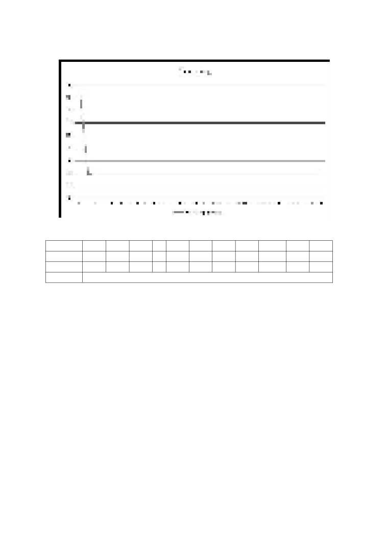
The data set we used is from Yale Face Database. We choose 136 images to analysis. When
we run our algorithm we need to divide it into two phases. First, we need to train our algorithm.
The purpose of this phase is to determine the minimum error which will be used in the next phase.
So we must ensure that the algorithm can converge at a certain point. During the training process,
the error will be reduced until it becomes a constant. The constant will be used as a threshold in
the next step. Figure 1 shows the error will not change after repeating 4 times. So the best error is
4. The horizontal axis represents the number of iterations, and the vertical axis represents error.
Seconds, we can use the constant obtained from the first step as the threshold to judge
whether the algorithm can stop. Table II shows when the training process is successful the time
consumed by the algorithm. In the table, “yes” represents the algorithm is succeed, in contrast
“no” represents the algorithm is failed. We can see that the average time used by the algorithm is
12374.3 milliseconds. The reason why the algorithm is failed is it fell into the local optimum.
Fig 6 the process of training
Table II time consumed by the algorithm
1
2
3
4
5
6
7
8
9
10
11
result
yes
yes
yes
no
yes
no
yes
yes
yes
yes
yes
time/ms
11642
23163
11615
11794
11715
11966
11687
11633
11892
11636
average/ms
12874.3
4.4 Theoretically Analysis of The Maximal Speedup
By measuring the time overhead of training, especially the average time of t1
, t2 and t3,
the maximal speedup and speed-up efficiency are listed below:
Time of serial execution: 5317.000000
Time of parallel execution :2665.000000
speed-up ratio
:1.995122
Speed-up efficiency
:0.997561
5. CONCLUSION
In this work, we accomplish face recognition by using deep learning algorithm. We mainly
apply the algorithm of convolution neural network to excavate the deep information of multi-layer
network in the process of face recognition .And we also utilize the algorithm to make parallel
computing on the cloud platform for accelerating the process of face recognition, analyzing
theoretical acceleration ratio, and experimental verification. Experimental results show that we
have achieved good results. Of course, the parallelism we do is coarse-grained, and there are still
many modules that can be fine-grained in the algorithm. This will be the focus for us in the future
to continue to improve the work.
ACKNOWLEDGMENT
During the time we work together to complete the course task, Prof. Chen takes much effort to
offer us guide and help. So the first person we must offer our thanks to is Mr.Chen. At the same
time, our major team leader Tianyi Liu, also deserves our sincerest thanks. He has done much
work to organize teammates and coordinate everyone’s work. And lastly,thanks to everybody in
our team, we reach a consensus and we make concerted efforts, then we can complete our work in
time and publish it on the website .
REFERENCES
[1] Lecun Y, Bottou L, Bengio Y, et al. Gradient-based learning applied to document recognition[
J]. Proceedings of the IEEE, 1998, 86(11):2278 - 2324.
[2] Dan C. Ciresan, Ueli Meier, Jonathan Masci, et al. Flexible, High Performance Convolutional
Neural Networks for Image Classification[J]. PROCEEDINGS OF THE TWENTY-SECOND IN
TERNATIONAL JOINT CONFERENCE ON ARTIFICIAL INTELLIGENCE, 2011.
[3] Hinton A K I S G. ImageNet classification with deep convolutional neural networks,” NIPS[J].
Advances in Neural Information Processing Systems, 2012:2012.
[4] Yadan O, Adams K, Taigman Y, et al. Multi-GPU Training of ConvNets[J]. Eprint Arxiv, 201
3.
[5] Lei Y, Ferrer L, Lawson A, et al. Application of convolutional neural networks to language ide
ntification in noisy conditions[C]//Proc. Speaker Odyssey Workshop (submitted). 2014.
[6] Sun Y, Wang X, Tang X. Deep Convolutional Network Cascade for Facial Point Detection[C]/
/ Computer Vision and Pattern Recognition (CVPR), 2013 IEEE Conference on. IEEE, 2013:3476
-3483.
[7] Abdel-Hamid O, Mohamed A R, Jiang H, et al. Applying Convolutional Neural Networks con
cepts to hybrid NN-HMM model for speech recognition[C]// Acoustics, Speech and Signal Proces
sing (ICASSP), 2012 IEEE International Conference on. IEEE, 2012:4277 - 4280.
[8] Boureau Y L, Ponce J, Lecun Y. A Theoretical Analysis of Feature Pooling in Visual Recognit
ion[J]. International Conference on Machine Learning Haifa Israel, 2010:111-118.
[9] Lecun Y, Kavukcuoglu K, Farabet C. Convolutional networks and applications in vision[C]//
Circuits and Systems (ISCAS), Proceedings of 2010 IEEE International Symposium on. IEEE, 20
10:253 - 256.
[10] Lecun P S. Convolutional Neural Networks Applied to HouseNumbers Digit Classification[C]
// Pattern Recognition (ICPR), 2012 21st International Conference on. IEEE, 2012:3288 - 3291.
[11] Goodfellow I J, Bulatov Y, Ibarz J, et al. Multi-digit number recognition from street view ima
gery using deep convolutional neural networks[J]. arXiv preprint arXiv:1312.6082, 2013.


