Rich feature hierarchies for accurate object detection and semantic segmentation
Author: R. Girshick, J. Donahue, T. Darrell, J. Malik, UC Berkeley and ICSI
Source: IEEE Conference on Computer Vision and Pattern Recognition 2014
Abstract
Object detection performance, as measured on the canonical PASCAL VOC dataset, has plateaued in the last few years. The best-performing methods are complex ensemble systems that typically combine multiple low-levelimage features with high-level context. In this paper, we propose a simple and scalable detection algorithm that improves mean average precision (mAP) by more than 30% relative to the previous best result on VOC 2012—achieving a mAP of 53.3%. Our approach combines two key insights: localize and segment objects and (2) when labeled training data is scarce, supervised pre-training for an auxiliary task, followed by domain-specific fine-tuning, yields a significant performance boost. Since we combine region proposals with CNNs, we call our method R-CNN: Regions with CNN features. We also present experiments that provide insight into what the network learns, revealing a rich hierarchy of image features. Source code for the complete system is available at Source code for the complete system is available at [link].
1. Introduction
Features matter. The last decade of progress on various visual recognition tasks has been based considerably on the use of SIFT [26] and HOG [7]. But if we look at performance on the canonical visual recognition task, PASCAL VOC object detection [12], it is generally acknowledged that progress has been slow during 2010-2012, with small gains obtained by building ensemble systems and employing minor variants of successful methods.
SIFT and HOG are blockwise orientation histograms, a representation we could associate roughly with complex cells in V1, the first cortical area in the primate visual pathway. But we also know that recognition occurs several stages downstream, which suggests that there might be hierarchical, multi-stage processes for computing features that are even more informative for visual recognition.
Fukushima’s “neocognitron” [16], a biologically-inspired hierarchical and shift-invariant model for pattern recognition, was an early attempt at just such a process. The neocognitron, however, lacked a supervised training algorithm. LeCun et al. [23] provided the missing algorithm by showing that stochastic gradient descent, via backpropagation, can train convolutional neural networks (CNNs), a class of models that extend the neocognitron.
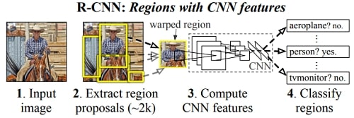
Figure 1: Object detection system overview. Our system (1) takes an input image, (2) extracts around 2000 bottom-up region proposals, (3) computes features for each proposal using a large convolutional neural network (CNN), and then (4) classifies each region using class-specific linear SVMs. R-CNN achieves a mean average precision (mAP) of 53.7% on PASCAL VOC 2010. For comparison, [32] reports 35.1% mAP using the same region proposals, but with a spatial pyramid and bag-of-visual-words approach. The popular deformable part models perform at 33.4%.
CNNs saw heavy use in the 1990s (e.g., [24]), but then fell out of fashion, particularly in computer vision, with the rise of support vector machines. In 2012, Krizhevsky et al. [22] rekindled interest in CNNs by showing substantially higher image classification accuracy on the ImageNet Large Scale Visual Recognition Challenge (ILSVRC) [9, 10]. Their success resulted from training a large CNN on 1.2 million labeled images, together with a few twists on LeCun’s CNN (e.g., max(x, 0) rectifying non-linearities and “dropout” regularization).
The significance of the ImageNet result was vigorously debated during the ILSVRC 2012 workshop. The central issue can be distilled to the following: To what extent do the CNN classification results on ImageNet generalize to object detection results on the PASCAL VOC Challenge?
We answer this question decisively by bridging the chasm between image classification and object detection. This paper is the first to show that a CNN can lead to dramatically higher object detection performance on PASCAL VOC as compared to systems based on simpler HOG-like features. Achieving this result required solving two problems: localizing objects with a deep network and training a high-capacity model with only a small quantity of annotated detection data.
Unlike image classification, detection requires localizing (likely many) objects within an image. One approach frames localization as a regression problem. However, work from Szegedy et al. [31]], concurrent with our own, indicates that this strategy may not fare well in practice (they report a mAP of 30.5% on VOC 2007 compared to the 58.5% achieved by our method). An alternative is to build a sliding-window detector. CNNs have been used in this way for at least two decades, typically on constrained object categories, such as faces [28], 33]] and pedestrians [29]]. In order to maintain high spatial resolution, these CNNs typically only have two convolutional and pooling layers. We also considered adopting a sliding-window approach. However, units high up in our network, which has five convolutional layers, have very large receptive fields (195 ✕ 195 pixels) and strides (32 ✕ 32 pixels) in the input image, which makes precise localization within the sliding-window paradigm an open technical challenge.
Instead, we solve the CNN localization problem by operating within the “recognition using regions” paradigm, as argued for by Gu et al. in [18]. At test-time, our method generates around 2000 category-independent region proposals for the input image, extracts a fixed-length feature vector from each proposal using a CNN, and then classifies each region with category-specific linear SVMs. We use a simple technique (affine image warping) to compute a fixed-size CNN input from each region proposal, regardless of the region’s shape. Figure 1 presents an overview of our method and highlights some of our results. Since our system combines region proposals with CNNs, we dub the method R-CNN: Regions with CNN features.
A second challenge faced in detection is that labeled data is scarce and the amount currently available is insufficient for training a large CNN. The conventional solution to this problem is to use unsupervised pre-training, followed by supervised fine-tuning (e.g., [29]). The second major contribution of this paper is to show that supervised pretraining on a large auxiliary dataset (ILSVRC), followed by domain-specific fine-tuning on a small dataset (PASCAL), is an effective paradigm for learning high-capacity CNNs when data is scarce. In our experiments, fine-tuning for detection improves mAP performance by 8 percentage points. After fine-tuning, our system achieves a mAP of 54% on VOC 2010 compared to 33% for the highly-tuned, HOGbased deformable part model (DPM) [14, 17].
Our system is also quite efficient. The only class-specific computations are a reasonably small matrix-vector product and greedy non-maximum suppression. This computational property follows from features that are shared across all categories and that are also two orders of magnitude lowerdimensional than previously used region features (cf. [32]]).
One advantage of HOG-like features is their simplicity: it’s easier to understand the information they carry (although [34]] shows that our intuition can fail us). Can we gain insight into the representation learned by the CNN? Perhaps the densely connected layers, with more than 54 million parameters, are the key? They are not. We “lobotomized” the CNN and found that a surprisingly large proportion, 94%, of its parameters can be removed with only a moderate drop in detection accuracy. Instead, by probing units in the network we see that the convolutional layers learn a diverse set of rich features (Figure 3).
Understanding the failure modes of our approach is also critical for improving it, and so we report results from the detection analysis tool of Hoiem et al. [20]]. As an immediate consequence of this analysis, we demonstrate that a simple bounding box regression method significantly reduces mislocalizations, which are the dominant error mode.
Before developing technical details, we note that because R-CNN operates on regions it is natural to extend it to the task of semantic segmentation. With minor modifications, we also achieve state-of-the-art results on the PASCAL VOC segmentation task, with an average segmentation accuracy of 47.9% on the VOC 2011 test set.
2. Object detection with R-CNN
Our object detection system consists of three modules. The first generates category-independent region proposals. These proposals define the set of candidate detections available to our detector. The second module is a large convolutional neural network that extracts a fixed-length feature decisions for each module, describe their test-time usage, detail how their parameters are learned, and show results on PASCAL VOC 2010-12.
2.1. Module design
Region proposals. A variety of recent papers offer methods for generating category-independent region proposals. Examples include: objectness [1], selective search [32], category-independent object proposals [11], constrained parametric min-cuts (CPMC) [5], multi-scale combinatorial grouping [3], and Ciresan et al. [6], who detect mitotic cells by applying a CNN to regularly-spaced square crops, which are a special case of region proposals. While R-CNN is agnostic to the particular region proposal method, we use selective search to enable a controlled comparison with prior detection work (e.g., [32], 35]]).

Figure 2: Warped training samples from VOC 2007 train.
Feature extraction. We extract a 4096-dimensional feature vector from each region proposal using the Caffe [21] implementation of the CNN described by Krizhevsky et al. [22]. Features are computed by forward propagating a mean-subtracted 227 ✕ 227 RGB image through five convolutional layers and two fully connected layers. We refer readers to [21, 22] for more network architecture details.
In order to compute features for a region proposal, we must first convert the image data in that region into a form that is compatible with the CNN (its architecture requires inputs of a fixed 227 ✕ 227 pixel size). Of the many possible transformations of our arbitrary-shaped regions, we opt for the simplest. Regardless of the size or aspect ratio of the candidate region, we warp all pixels in a tight bounding box around it to the required size. Prior to warping, we dilate the tight bounding box so that at the warped size there are exactly p pixels of warped image context around the original box (we use p = 16). Figure 2 shows a random sampling of warped training regions. The supplementary material discusses alternatives to warping.
2.2. Test-time detection
At test time, we run selective search on the test image to extract around 2000 region proposals (we use selective search’s “fast mode” in all experiments). We warp each proposal and forward propagate it through the CNN in order to read off features from the desired layer. Then, for each class, we score each extracted feature vector using the SVM trained for that class. Given all scored regions in an image, we apply a greedy non-maximum suppression (for each class independently) that rejects a region if it has an intersection-over-union (IoU) overlap with a higher scoring selected region larger than a learned threshold.
Run-time analysis. Two properties make detection efficient. First, all CNN parameters are shared across all categories. Second, the feature vectors computed by the CNN are low-dimensional when compared to other common approaches, such as spatial pyramids with bag-of-visual-word encodings. The features used in the UVA detection system [32], for example, are two orders of magnitude larger than ours (360k vs. 4k-dimensional).
The result of such sharing is that the time spent computing region proposals and features (13s/image on a GPU or 53s/image on a CPU) is amortized over all classes. The only class-specific computations are dot products between features and SVM weights and non-maximum suppression. In practice, all dot products for an image are batched into a single matrix-matrix product. The feature matrix is typically 2000 ✕ 4096 and the SVM weight matrix is 4096 ✕ N, where N is the number of classes.
This analysis shows that R-CNN can scale to thousands of object classes without resorting to approximate techniques, such as hashing. Even if there were 100k classes, the resulting matrix multiplication takes only 10 seconds on a modern multi-core CPU. This efficiency is not merely the result of using region proposals and shared features. The UVA system, due to its high-dimensional features, would be two orders of magnitude slower while requiring 134GB of memory just to store 100k linear predictors, compared to just 1.5GB for our lower-dimensional features.
It is also interesting to contrast R-CNN with the recent work from Dean et al. on scalable detection using DPMs and hashing [8]. They report a mAP of around 16% on VOC 2007 at a run-time of 5 minutes per image when introducing 10k distractor classes. With our approach, 10k detectors can run in about a minute on a CPU, and because no approximations are made mAP would remain at 59% (Section 3.2).
2.3. Training
Supervised pre-training. We discriminatively pre-trained the CNN on a large auxiliary dataset (ILSVRC 2012) with image-level annotations (i.e., no bounding box labels). Pretraining was performed using the open source Caffe CNN library [21]. In brief, our CNN nearly matches the performance of Krizhevsky et al. [22], obtaining a top-1 error rate 2.2 percentage points higher on the ILSVRC 2012 validation set. This discrepancy is due to simplifications in the training process.
Domain-specific fine-tuning. To adapt our CNN to the new task (detection) and the new domain (warped VOC windows), we continue stochastic gradient descent (SGD) training of the CNN parameters using only warped region proposals from VOC. Aside from replacing the CNN’s ImageNet-specific 1000-way classification layer with a randomly initialized 21-way classification layer (for the 20 VOC classes plus background), the CNN architecture is unchanged. We treat all region proposals with ≥ 0.5 IoU overlap with a ground-truth box as positives for that box’s class and the rest as negatives. We start SGD at a learning rate of 0.001 (1/10th of the initial pre-training rate), which allows fine-tuning to make progress while not clobbering the initialization. In each SGD iteration, we uniformly sample 32 positive windows (over all classes) and 96 background windows to construct a mini-batch of size 128. We bias the sampling towards positive windows because they are extremely rare compared to background.
Object category classifiers. Consider training a binary classifier to detect cars. It’s clear that an image region tightly enclosing a car should be a positive example. Similarly, it’s clear that a background region, which has nothing to do with cars, should be a negative example. Less clear is how to label a region that partially overlaps a car. We resolve this issue with an IoU overlap threshold, below which regions are defined as negatives. The overlap threshold, 0.3, was selected by a grid search over {0, 0.1, ... , 0.5} on a validation set. We found that selecting this threshold carefully is important. Setting it to 0.5, as in [32], decreased mAP by 5 points. Similarly, setting it to 0 decreased mAP by 4 points. Positive examples are defined simply to be the ground-truth bounding boxes for each class.
Once features are extracted and training labels are applied, we optimize one linear SVM per class. Since the training data is too large to fit in memory, we adopt the standard hard negative mining method [14, 30]. Hard negative mining converges quickly and in practice mAP stops increasing after only a single pass over all images.
In supplementary material we discuss why the positive and negative examples are defined differently in fine-tuning versus SVM training. We also discuss why it’s necessary to train detection classifiers rather than simply use outputs from the final layer (fc8) of the fine-tuned CNN.
2.4. Results on PASCAL VOC 2010-12
Following the PASCAL VOC best practices [12], we validated all design decisions and hyperparameters on the VOC 2007 dataset (Section 3.2). For final results on the VOC 2010-12 datasets, we fine-tuned the CNN on VOC 2012 train and optimized our detection SVMs on VOC 2012 trainval. We submitted test results to the evaluation server only once for each of the two major algorithm variants (with and without bounding box regression).
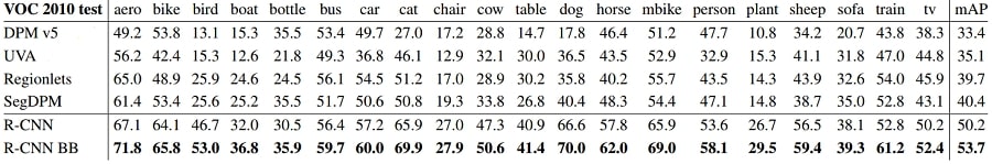
Table 1 shows complete results on VOC 2010. We compare our method against four strong baselines, including SegDPM [15], which combines DPM detectors with the output of a semantic segmentation system [4] and uses additional inter-detector context and image-classifier rescoring. The most germane comparison is to the UVA system from Uijlings et al. [12], since our systems use the same region proposal algorithm. To classify regions, their method builds a four-level spatial pyramid and populates it with densely sampled SIFT, Extended OpponentSIFT, and RGBSIFT descriptors, each vector quantized with 4000-word codebooks. Classification is performed with a histogram intersection kernel SVM. Compared to their multi-feature, non-linear kernel SVM approach, we achieve a large improvement in mAP, from 35.1% to 53.7% mAP, while also being much faster (Section 2.2). Our method achieves similar performance (53.3% mAP) on VOC 2011/12 test.
3. Visualization, ablation, and modes of error
3.1. Visualizing learned features
3.1. Visualizing learned features
First-layer filters can be visualized directly and are easy to understand [22]. They capture oriented edges and opponent colors. Understanding the subsequent layers is more challenging. Zeiler and Fergus present a visually attractive deconvolutional approach in [36]. We propose a simple (and complementary) non-parametric method that directly shows what the network learned.
The idea is to single out a particular unit (feature) in the network and use it as if it were an object detector in its own right. That is, we compute the unit’s activations on a large set of held-out region proposals (about 10 million), sort the proposals from highest to lowest activation, perform nonmaximum suppression, and then display the top-scoring regions. Our method lets the selected unit “speak for itself” by showing exactly which inputs it fires on. We avoid averaging in order to see different visual modes and gain insight into the invariances computed by the unit.
We visualize units from layer pool5, which is the maxpooled output of the network’s fifth and final convolutional layer. The pool5 feature map is 6 ✕ 6 ✕ 256 = 9216-dimensional. Ignoring boundary effects, each pool5 unit has a receptive field of 195 ✕ 195 pixels in the original 227 ✕ 227 pixel input. A central pool5 unit has a nearly global view, while one near the edge has a smaller, clipped support.
Each row in Figure 3 displays the top 16 activations for a pool5 unit from a CNN that we fine-tuned on VOC 2007 trainval. Six of the 256 functionally unique units are visualized (the supplementary material includes more). These units were selected to show a representative sample of what the network learns. In the second row, we see a unit that fires on dog faces and dot arrays. The unit corresponding to the third row is a red blob detector. There are also detectors for human faces and more abstract patterns such as text and triangular structures with windows. The network appears to learn a representation that combines a small number of class-tuned features together with a distributed representation of shape, texture, color, and material properties. The a large set of compositions of these rich features.
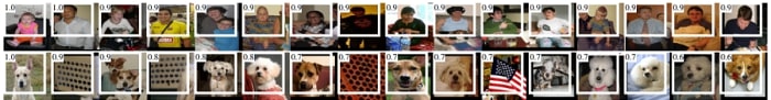
Figure 3: Top regions for six pool5 units. Receptive fields and activation values are drawn in white.
3.2. Ablation studies
Performance layer-by-layer, without fine-tuning. To understand which layers are critical for detection performance, we analyzed results on the VOC 2007 dataset for each of the CNN’s last three layers. Layer pool5 was briefly described in Section 3.1. The final two layers are summarized below.
Layer fc6 is fully connected to pool5. To compute features, it multiplies a 4096 ✕ 9216 weight matrix by the pool5 feature map (reshaped as a 9216-dimensional vector) and then adds a vector of biases. This intermediate vector is component-wise half-wave rectified (x ← max(0, x)).
Layer fc7 is the final layer of the network. It is implemented by multiplying the features computed by fc6 by a 4096 ✕ 4096 weight matrix, and similarly adding a vector of biases and applying half-wave rectification.
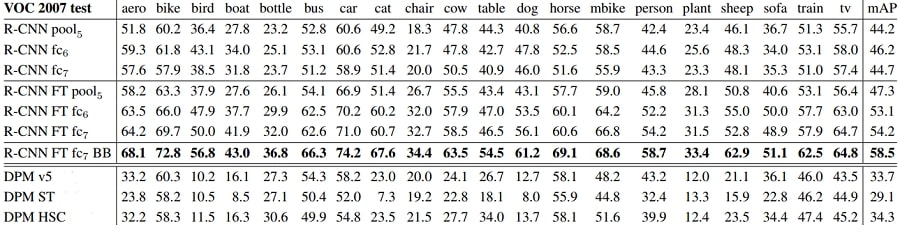
We start by looking at results from the CNN without fine-tuning on PASCAL, i.e. all CNN parameters were pretrained on ILSVRC 2012 only. Analyzing performance layer-by-layer (Table 2 rows 1-3) reveals that features from fc7 generalize worse than features from fc6. This means that 29%, or about 16.8 million, of the CNN’s parameters can be removed without degrading mAP. More surprising is that removing both fc7 and fc6 produces quite good results even though pool5 features are computed using only 6% of the CNN’s parameters. Much of the CNN’s representational power comes from its convolutional layers, rather than from the much larger densely connected layers. This finding suggests potential utility in computing a dense feature map, in the sense of HOG, of an arbitrary-sized image by using only the convolutional layers of the CNN. This representation would enable experimentation with sliding-window detectors, including DPM, on top of pool5 features.
Performance layer-by-layer, with fine-tuning. We now look at results from our CNN after having fine-tuned its parameters on VOC 2007 trainval. The improvement is striking (Table 2 rows 4-6): fine-tuning increases mAP by 8.0 percentage points to 54.2%. The boost from fine-tuning is much larger for fc6 and fc7 than for pool5, which suggests that the pool5 features learned from ImageNet are general and that most of the improvement is gained from learning domain-specific non-linear classifiers on top of them.
Comparison to recent feature learning methods. Relatively few feature learning methods have been tried on PASCAL VOC detection. We look at two recent approaches that build on deformable part models. For reference, we also include results for the standard HOG-based DPM [17].
The first DPM feature learning method, DPM ST [25], augments HOG features with histograms of “sketch token” probabilities. Intuitively, a sketch token is a tight distribution of contours passing through the center of an image patch. Sketch token probabilities are computed at each pixel by a random forest that was trained to classify 35 ✕ 35 pixel patches into one of 150 sketch tokens or background.
The second method, DPM HSC [27], replaces HOG with histograms of sparse codes (HSC). To compute an HSC, sparse code activations are solved for at each pixel using a learned dictionary of 100 7 ✕ 7 pixel (grayscale) atoms. The resulting activations are rectified in three ways (full and both half-waves), spatially pooled, unit l2 normalized, and then power transformed (x ← sign(x)|x|α).
All R-CNN variants strongly outperform the three DPM baselines (Table 2 rows 8-10), including the two that use feature learning. Compared to the latest version of DPM, which uses only HOG features, our mAP is more than 20 percentage points higher: 54.2% vs. 33.7%-a 61% relative improvement. The combination of HOG and sketch tokens yields 2.5 mAP points over HOG alone, while HSC improves over HOG by 4 mAP points (when compared internally to their private DPM baselines-both use nonpublic implementations of DPM that underperform the open source version [17]). These methods achieve mAPs of 29.1% and 34.3%, respectively
3.3. Detection error analysis
We applied the excellent detection analysis tool from Hoiem et al. [20] in order to reveal our method’s error modes, understand how fine-tuning changes them, and to see how our error types compare with DPM. A full summary of the analysis tool is beyond the scope of this paper and we encourage readers to consult [20] to understand some finer details (such as “normalized AP”). Since the analysis is best absorbed in the context of the associated plots, we present the discussion within the captions of Figure 4 and Figure 5.
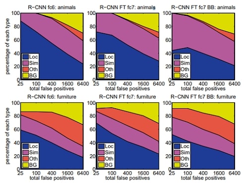
Figure 4: Distribution of top-ranked false positive (FP) types. Each plot shows the evolving distribution of FP types as more FPs are considered in order of decreasing score. Each FP is categorized into 1 of 4 types: Loc—poor localization (a detection with an IoU overlap with the correct class between 0.1 and 0.5, or a duplicate); Sim—confusion with a similar category; Oth—confusion with a dissimilar object category; BG—a FP that fired on background. Compared with DPM (see [20]), significantly more of our errors result from poor localization, rather than confusion with background or other object classes, indicating that the CNN features are much more discriminative than HOG. Loose localization likely results from our use of bottom-up region proposals and the positional invariance learned from pre-training the CNN for whole-image classification. Column three shows how our simple bounding box regression method fixes many localization errors.
References
- B. Alexe, T. Deselaers, and V. Ferrari. Measuring the objectness of image windows. TPAMI, 2012.
- P. Arbelaez, B. Hariharan, C. Gu, S. Gupta, L. Bourdev, and J. Malik. Semantic segmentation using regions and parts. In CVPR, 2012.
- P. Arbelaez, J. Pont-Tuset, J. Barron, F. Marques, and J. Malik. Multiscale combinatorial grouping. In CVPR, 2014.
- J. Carreira, R. Caseiro, J. Batista, and C. Sminchisescu. Semantic segmentation with second-order pooling. In ECCV, 2012.
- J. Carreira and C. Sminchisescu. CPMC: Automatic object segmentation using constrained parametric min-cuts. TPAMI, 2012.
- D. Ciresan, A. Giusti, L. Gambardella, and J. Schmidhuber. Mitosis detection in breast cancer histology images with deep neural networks. In MICCAI, 2013.
- N. Dalal and B. Triggs. Histograms of oriented gradients for human detection. In CVPR, 2005.
- T. Dean, M. A. Ruzon, M. Segal, J. Shlens, S. Vijayanarasimhan, and J. Yagnik. Fast, accurate detection of 100,000 object classes on a single machine. In CVPR, 2013.
- J. Deng, A. Berg, S. Satheesh, H. Su, A. Khosla, and L. Fei-Fei. ImageNet Large Scale Visual Recognition Competition 2012 (ILSVRC2012).
- J. Deng, W. Dong, R. Socher, L.-J. Li, K. Li, and L. Fei-Fei. ImageNet: A large-scale hierarchical image database. In CVPR, 2009.
- I. Endres and D. Hoiem. Category independent object proposals. In ECCV, 2010.
- M. Everingham, L. Van Gool, C. K. I. Williams, J. Winn, and A. Zisserman. The PASCAL Visual Object Classes (VOC) Challenge. IJCV, 2010.
- C. Farabet, C. Couprie, L. Najman, and Y. LeCun. Learning hierarchical features for scene labeling. TPAMI, 2013.
- P. Felzenszwalb, R. Girshick, D. McAllester, and D. Ramanan. Object detection with discriminatively trained part based models. TPAMI, 2010.
- S. Fidler, R. Mottaghi, A. Yuille, and R. Urtasun. Bottom-up segmentation for top-down detection. In CVPR, 2013.
- K. Fukushima. Neocognitron: A self-organizing neural network model for a mechanism of pattern recognition unaffected by shift in position. Biological cybernetics, 36(4):193–202, 1980.
- R. Girshick, P. Felzenszwalb, and D. McAllester. Discriminatively trained deformable part models, release 5.
- C. Gu, J. J. Lim, P. Arbelaez, and J. Malik. Recognition using regions. In CVPR, 2009.
- B. Hariharan, P. Arbelaez, L. Bourdev, S. Maji, and J. Malik. Semantic contours from inverse detectors. In ICCV, 2011.
- D. Hoiem, Y. Chodpathumwan, and Q. Dai. Diagnosing error in object detectors. In ECCV. 2012.
- Y. Jia. Caffe: An open source convolutional architecture for fast feature embedding.
- A. Krizhevsky, I. Sutskever, and G. Hinton. ImageNet classification with deep convolutional neural networks. In NIPS, 2012.
- Y. LeCun, B. Boser, J. Denker, D. Henderson, R. Howard, W. Hubbard, and L. Jackel. Backpropagation applied to handwritten zip code recognition. Neural Comp., 1989.
- Y. LeCun, L. Bottou, Y. Bengio, and P. Haffner. Gradient-based learning applied to document recognition. Proc. of the IEEE, 1998.
- J. J. Lim, C. L. Zitnick, and P. Dollar. Sketch tokens: A learned mid-level representation for contour and object detection. In CVPR, 2013.
- D. Lowe. Distinctive image features from scale-invariant keypoints. IJCV, 2004.
- X. Ren and D. Ramanan. Histograms of sparse codes for object detection. In CVPR, 2013.