Fast R-CNN
Author: R. Girshick
Source: Proceedings of the IEEE International Conference on Computer Vision 2015, Pages 1440-1448
Abstract
This paper proposes a Fast Region-based Convolutional Network method (Fast R-CNN) for object detection. Fast R-CNN builds on previous work to efficiently classify object proposals using deep convolutional networks. Compared to previous work, Fast R-CNN employs several innovations to improve training and testing speed while also increasing detection accuracy. Fast R-CNN trains the very deep VGG16 network 9✕ faster than R-CNN, is 213✕ faster at test-time, and achieves a higher mAP on PASCAL VOC 2012. Compared to SPPnet, Fast R-CNN trains VGG16 3✕ faster, tests 10✕ faster, and is more accurate
1. Introduction
Recently, deep ConvNets have significantly improved image classification and object detection [9] accuracy. Compared to image classification, object detection is a more challenging task that requires more complex methods to solve. Due to this complexity, current approaches (e.g., [9, 11]) train models in multi-stage pipelines that are slow and inelegant.
Complexity arises because detection requires the accurate localization of objects, creating two primary challenges. First, numerous candidate object locations (often called “proposals”) must be processed. Second, these candidates provide only rough localization that must be refined to achieve precise localization. Solutions to these problems often compromise speed, accuracy, or simplicity
In this paper, we streamline the training process for stateof-the-art ConvNet-based object detectors [9, 11]. We propose a single-stage training algorithm that jointly learns to classify object proposals and refine their spatial locations.
The resulting method can train a very deep detection network (VGG16) 9✕ faster than R-CNN [9] and 3✕ faster than SPPnet [11]. At runtime, the detection network processes images in 0.3s (excluding object proposal time) while achieving top accuracy on PASCAL VOC 2012 [7] with a mAP of 66% (vs. 62% for R-CNN).
1.1. R-CNN and SPPnet
The Region-based Convolutional Network method (RCNN) [9] achieves excellent object detection accuracy by using a deep ConvNet to classify object proposals. R-CNN, however, has notable drawbacks:
- Training is a multi-stage pipeline. R-CNN first finetunes a ConvNet on object proposals using log loss. Then, it fits SVMs to ConvNet features. These SVMs act as object detectors, replacing the softmax classifier learnt by fine-tuning. In the third training stage, bounding-box regressors are learned.
- Training is expensive in space and time. For SVM and bounding-box regressor training, features are extracted from each object proposal in each image and written to disk. With very deep networks, such as VGG16, this process takes 2.5 GPU-days for the 5k images of the VOC07 trainval set. These features require hundreds of gigabytes of storage.
- Object detection is slow. At test-time, features are extracted from each object proposal in each test image. Detection with VGG16 takes 47s / image (on a GPU).
R-CNN is slow because it performs a ConvNet forward pass for each object proposal, without sharing computation. Spatial pyramid pooling networks (SPPnets) [11] were proposed to speed up R-CNN by sharing computation. The SPPnet method computes a convolutional feature map for the entire input image and then classifies each object proposal using a feature vector extracted from the shared feature map. Features are extracted for a proposal by maxpooling the portion of the feature map inside the proposal into a fixed-size output (e.g., 6 ✕ 6). Multiple output sizes are pooled and then concatenated as in spatial pyramid pooling. SPPnet accelerates R-CNN by 10 to 100✕ at test time. Training time is also reduced by 3✕ due to faster proposal feature extraction.
SPPnet also has notable drawbacks. Like R-CNN, training is a multi-stage pipeline that involves extracting features, fine-tuning a network with log loss, training SVMs, and finally fitting bounding-box regressors. Features are also written to disk. But unlike R-CNN, the fine-tuning algorithm proposed in [11] cannot update the convolutional layers that precede the spatial pyramid pooling. Unsurprisingly, this limitation (fixed convolutional layers) limits the accuracy of very deep networks.
1.2. Contributions
We propose a new training algorithm that fixes the disadvantages of R-CNN and SPPnet, while improving on their speed and accuracy. We call this method Fast R-CNN because it’s comparatively fast to train and test. The Fast RCNN method has several advantages:
- Higher detection quality (mAP) than R-CNN, SPPnet
- Training is single-stage, using a multi-task loss
- Training can update all network layers
- No disk storage is required for feature caching
Fast R-CNN is written in Python and C++ (Caffe [13]) and is available under the open-source MIT License at [link].
2. Fast R-CNN architecture and training
Fig. 1 illustrates the Fast R-CNN architecture. A Fast R-CNN network takes as input an entire image and a set of object proposals. The network first processes the whole image with several convolutional (conv) and max pooling layers to produce a conv feature map. Then, for each object proposal a region of interest (RoI) pooling layer extracts a fixed-length feature vector from the feature map. Each feature vector is fed into a sequence of fully connected (fc) layers that finally branch into two sibling output layers: one that produces softmax probability estimates over K object classes plus a catch-all “background” class and another layer that outputs four real-valued numbers for each of the K object classes. Each set of 4 values encodes refined bounding-box positions for one of the K classes.
2.1. The RoI pooling layer
The RoI pooling layer uses max pooling to convert the features inside any valid region of interest into a small feature map with a fixed spatial extent of H ✕ W (e.g., 7 ✕ 7), where H and W are layer hyper-parameters that are independent of any particular RoI. In this paper, an RoI is a rectangular window into a conv feature map. Each RoI is defined by a four-tuple (r, c, h, w) that specifies its top-left corner (r, c) and its height and width (h, w).
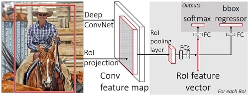
Figure 1. Fast R-CNN architecture. An input image and multiple regions of interest (RoIs) are input into a fully convolutional network. Each RoI is pooled into a fixed-size feature map and then mapped to a feature vector by fully connected layers (FCs). The network has two output vectors per RoI: softmax probabilities and per-class bounding-box regression offsets. The architecture is trained end-to-end with a multi-task loss.
RoI max pooling works by dividing the h ✕ w RoI window into an H ✕ W grid of sub-windows of approximate size h/H ✕ w/W and then max-pooling the values in each sub-window into the corresponding output grid cell. Pooling is applied independently to each feature map channel, as in standard max pooling. The RoI layer is simply the special-case of the spatial pyramid pooling layer used in SPPnets [11] in which there is only one pyramid level. We use the pooling sub-window calculation given in [11].
2.2. Initializing from pre-trained networks
We experiment with three pre-trained ImageNet [4] networks, each with five max pooling layers and between five and thirteen conv layers (see Section 4.1 for network details). When a pre-trained network initializes a Fast R-CNN network, it undergoes three transformations.
First, the last max pooling layer is replaced by a RoI pooling layer that is configured by setting H and W to be compatible with the net’s first fully connected layer (e.g., H = W = 7 for VGG16).
Second, the network’s last fully connected layer and softmax (which were trained for 1000-way ImageNet classification) are replaced with the two sibling layers described earlier (a fully connected layer and softmax over K + 1 categories and category-specific bounding-box regressors).
Third, the network is modified to take two data inputs: a list of images and a list of RoIs in those images.
2.3. Fine-tuning for detection
Training all network weights with back-propagation is an important capability of Fast R-CNN. First, let’s elucidate why SPPnet is unable to update weights below the spatial pyramid pooling layer.
The root cause is that back-propagation through the SPP layer is highly inefficient when each training sample (i.e. RoI) comes from a different image, which is exactly how R-CNN and SPPnet networks are trained. The inefficiency stems from the fact that each RoI may have a very large receptive field, often spanning the entire input image. Since the forward pass must process the entire receptive field, the training inputs are large (often the entire image).
We propose a more efficient training method that takes advantage of feature sharing during training. In Fast RCNN training, stochastic gradient descent (SGD) minibatches are sampled hierarchically, first by sampling N images and then by sampling R/N RoIs from each image. Critically, RoIs from the same image share computation and memory in the forward and backward passes. Making N small decreases mini-batch computation. For example, when using N = 2 and R = 128, the proposed training scheme is roughly 64✕ faster than sampling one RoI from 128 different images (i.e., the R-CNN and SPPnet strategy).
One concern over this strategy is it may cause slow training convergence because RoIs from the same image are correlated. This concern does not appear to be a practical issue and we achieve good results with N = 2 and R = 128 using fewer SGD iterations than R-CNN.
In addition to hierarchical sampling, Fast R-CNN uses a streamlined training process with one fine-tuning stage that jointly optimizes a softmax classifier and bounding-box regressors, rather than training a softmax classifier, SVMs, and regressors in three separate stages [9, 11]. The components of this procedure (the loss, mini-batch sampling strategy, back-propagation through RoI pooling layers, and SGD hyper-parameters) are described below.
Multi-task loss. A Fast R-CNN network has two sibling output layers. The first outputs a discrete probability distribution (per RoI), p = (p0, ... , pK), over K + 1 categories. As usual, p is computed by a softmax over the K + 1 outputs of a fully connected layer. The second sibling layer outputs bounding-box regression offsets, tk = (tkx, tky, tkw, tkh), for each of the K object classes, indexed by k. We use the parameterization for tk given in [9], in which tk specifies a scale-invariant translation and log-space height/width shift relative to an object proposal
Each training RoI is labeled with a ground-truth class u and a ground-truth bounding-box regression target v. We use a multi-task loss L on each labeled RoI to jointly train for classification and bounding-box regression
in which Lcls(p, u) = -log pu is log loss for true class u.
The second task loss, Lloc, is defined over a tuple of true bounding-box regression targets for class u, v = (vx, vy, vw, vh), and a predicted tuple tu = (tux, tuy, tuw, tuh), again for class u. The Iverson bracket indicator function [u ≥ 1] evaluates to 1 when u ≥ 1 and 0 otherwise. By convention the catch-all background class is labeled u = 0. For background RoIs there is no notion of a ground-trut bounding box and hence Lloc is ignored. For bounding-box regression, we use the loss
in which
is a robust L1 loss that is less sensitive to outliers than the L2 loss used in R-CNN and SPPnet. When the regression targets are unbounded, training with L2 loss can require careful tuning of learning rates in order to prevent exploding gradients. Eq. 3 eliminates this sensitivity.
3. Main results
Three main results support this paper’s contributions:
- State-of-the-art mAP on VOC07, 2010, and 2012
- Fast training and testing compared to R-CNN, SPPnet
- Fine-tuning conv layers in VGG16 improves mAP
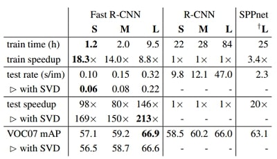
Fast training and testing times are our second main result. Table 4 compares training time (hours), testing rate (seconds per image), and mAP on VOC07 between Fast RCNN, R-CNN, and SPPnet. For VGG16, Fast R-CNN processes images 146✕ faster than R-CNN without truncated SVD and 213✕ faster with it. Training time is reduced by 9✕, from 84 hours to 9.5. Compared to SPPnet, Fast RCNN trains VGG16 2.7✕ faster (in 9.5 vs. 25.5 hours) and tests 7✕ faster without truncated SVD or 10✕ faster with it. Fast R-CNN also eliminates hundreds of gigabytes of disk storage, because it does not cache features.
Table 1. Runtime comparison between the same models in Fast RCNN, R-CNN, and SPPnet. Fast R-CNN uses single-scale mode. SPPnet uses the five scales specified in [11]. Timing provided by the authors of [11]. Times were measured on an Nvidia K40 GPU.
Truncated SVD. Truncated SVD can reduce detection time by more than 30% with only a small (0.3 percentage point) drop in mAP and without needing to perform additional fine-tuning after model compression. Fig. 2 illustrates how using the top 1024 singular values from the 25088 ✕ 4096 matrix in VGG16’s fc6 layer and the top 256 singular values from the 4096 ✕ 4096 fc7 layer reduces runtime with little loss in mAP. Further speed-ups are possible with smaller drops in mAP if one fine-tunes again after.
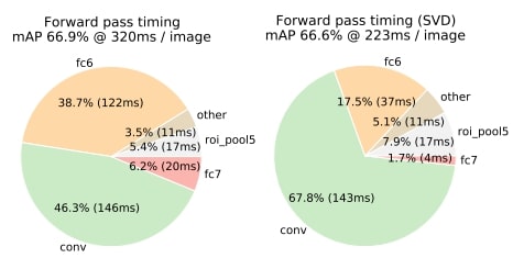
Figure 2. Timing for VGG16 before and after truncated SVD. Before SVD, fully connected layers fc6 and fc7 take 45% of the time.
4. Conclusion
This paper proposes Fast R-CNN, a clean and fast update to R-CNN and SPPnet. In addition to reporting state-of-theart detection results, we present detailed experiments that we hope provide new insights. Of particular note, sparse object proposals appear to improve detector quality. This issue was too costly (in time) to probe in the past, but becomes practical with Fast R-CNN. Of course, there may exist yet undiscovered techniques that allow dense boxes to perform as well as sparse proposals. Such methods, if developed, may help further accelerate object detection.
References
- J. Carreira, R. Caseiro, J. Batista, and C. Sminchisescu. Semantic segmentation with second-order pooling. In ECCV, 2012.
- R. Caruana. Multitask learning. Machine learning, 28(1), 1997.
- K. Chatfield, K. Simonyan, A. Vedaldi, and A. Zisserman. Return of the devil in the details: Delving deep into convolutional nets. In BMVC, 2014.
- J. Deng, W. Dong, R. Socher, L.-J. Li, K. Li, and L. FeiFei. ImageNet: A large-scale hierarchical image database. In CVPR, 2009.
- E. Denton, W. Zaremba, J. Bruna, Y. LeCun, and R. Fergus. Exploiting linear structure within convolutional networks for efficient evaluation. In NIPS, 2014.
- D. Erhan, C. Szegedy, A. Toshev, and D. Anguelov. Scalable object detection using deep neural networks. In CVPR, 2014.
- M. Everingham, L. Van Gool, C. K. I. Williams, J. Winn, and A. Zisserman. The PASCAL Visual Object Classes (VOC) Challenge. IJCV, 2010.
- P. Felzenszwalb, R. Girshick, D. McAllester, and D. Ramanan. Object detection with discriminatively trained part based models. TPAMI, 2010.
- R. Girshick, J. Donahue, T. Darrell, and J. Malik. Rich feature hierarchies for accurate object detection and semantic segmentation. In CVPR, 2014.
- R. Girshick, J. Donahue, T. Darrell, and J. Malik. Regionbased convolutional networks for accurate object detection and segmentation. TPAMI, 2015.
- K. He, X. Zhang, S. Ren, and J. Sun. Spatial pyramid pooling in deep convolutional networks for visual recognition. In ECCV, 2014.
- J. H. Hosang, R. Benenson, P. Dollar, and B. Schiele. What makes for effective detection proposals?
- Y. Jia, E. Shelhamer, J. Donahue, S. Karayev, J. Long, R. Girshick, S. Guadarrama, and T. Darrell. Caffe: Convolutional architecture for fast feature embedding. In Proc. of the ACM International Conf. on Multimedia, 2014.