Contents
- Introduction
- 1. The choice of means and methods for the implementation of the task
- 1.1 Choosing an algorithm
- 1.2 Hardware Selection
- 1.3 Software selection
- 2. Object modeling
- 3. Solution of the inverse problem of kinematics
- 4. Computer vision tools used to solve the sorting problem
- Conclusions
- List of sources
Introduction
One of the most important and urgent directions in the development of robotics is the development of manipulators equipped with technical vision. The relevance of this direction is due to the fact that such robots can replace monotonous human labor and facilitate the performance of work in harmful or dangerous conditions.
The aim of this work is to create a vision prototype for a robotic sorter.
To achieve this goal, it is necessary to ensure the solution of the following tasks: analysis and selection of hardware and software, selection of a method for solving the inverse kinematics problem, as well as its direct solution, software implementation of the vision algorithm.
Computer vision (aka technical vision) is the theory and technology of creating machines that can detect, track and classify objects.
Robots–manipulators are automatic or operator-controlled devices that perform a specified range of operations instead of a person.
Initially, manipulators were created to work in hazardous facilities and conditions where a person is physically unable to perform the assigned tasks — for example, under water, in aggressive gas, radiation environments, vacuum, with the threat of a spill of harmful chemicals.
The capabilities of robots and their advantages over manual labor have provided devices with rapid distribution and popularity in all areas — from nuclear technology to educational programs. At the moment, manipulators are most actively involved in industry, in almost all of its areas — it is there that there is a very high need for automation and reducing the role of manual labor. Using an industrial robot increases production efficiency and minimizes errors and rejects.
1. The choice of means and methods for the implementation of the task
1.1 Choice of algorithm
In general, a vision system works according to the following principle: a camera or any other optical system (lidar, thermal imager) perceives information about the observed space or object, transmits it to a computing device that processes the image and generates a control signal to the actuator.
As an executive device, we have a six-link manipulator. Sorting will take place on a flat, stationary surface.
Based on the conditions, we can form a sequence of actions to solve the problem. The camera transmits the image to a single-board computer, which, analyzing the received frame, selects individual objects, classifies them and calculates coordinates to capture details. Then, the obtained coordinates are sent to the unit for calculating the inverse kinematics problem to find the angular coordinates of the manipulator links. After that, based on the received data, a control signal is generated. This process is cyclical and repeats until the working surface is "free" of the desired parts. If they are found again, the process starts again.
1.2 Hardware Selection
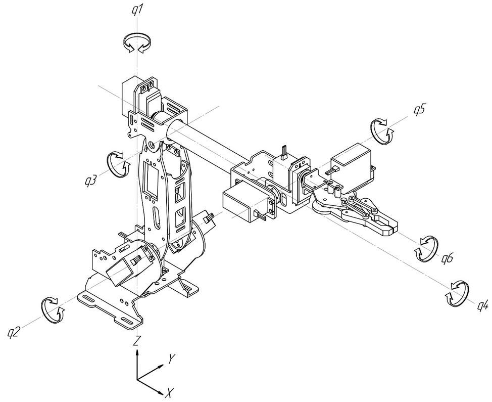
Having decided on the way to solve the problem, it is necessary to choose hardware and software for its implementation. As already mentioned, a six–link manipulator is used as a working body, the kinematic diagram of which is shown in Figure 1.2.

Figure 1.1 – Kinematic diagram of the sorter robot
This structure is often used in industry, as it can be used for a wide range of tasks due to the large number of moving parts. Moreover, it does not have excessive degrees of freedom, which facilitates the solution of the inverse problem of kinematics.
Eight DS3218 servo motors are used to drive the manipulator.
The torque of these motors is enough to provide the required lifting capacity of the manipulator. Provided that two motors are used to move the second link (the most loaded). Also, the choice of these motors is due to their availability, wide angle of rotation and good wear resistance.
Servo motors are controlled by regulating the duty cycle of the pulse width modulation (PWM) signal [1].
Conventional microcontrollers are not suitable for streaming image processing and solving the inverse kinematics problem. These tasks require significant processing power. Therefore, a single–board computer Raspberry Pi 4 is used as a computing device in this work. Its main advantages are: small size, low power consumption, full–fledged operating system, free software, low price. With its hardware I/O ports, it allows you to program real devices, physical systems, and objects [2].
Unfortunately, the Raspberry Pi 4 has only two hardware–supported PWM channels, and software solutions will not provide the required signal quality to control servo motors. This problem is solved by using an external PWM module. In this work, the PCA9685 module is used, which also provides galvanic isolation. It is a 16–channel 12–bit controller with an adjustable PWM frequency from 24 to 1526 Hz. To control the PCA9685, the I2C bus is used, this board has two groups of I2C bus connectors on both sides. This allows you to connect several cards in series on one bus or connect other I2C devices [3].
The power supply of the controller and the outputs of the PWM channels is divided and can be from 3 to 5 V. For PWM channels, a maximum voltage of 6 V.
1.3 Software Selection
For the software implementation of vision algorithms and solving the inverse kinematics problem, the Python programming language and the open source computer vision library OpenCV were chosen. OpenCV is free to use for academic and commercial purposes [4].
The choice in favor of this software was made due to the simplicity and availability of these tools. OpenCV is widely used in many tasks related to the creation of computer vision systems, as it has a wide range of tools for image processing.
To solve the inverse problem of kinematics, the NumPy and SciPy libraries are used. The NumPy library allows you to simplify matrix calculations, so that similar code in the C++ programming language will take significantly more lines, and therefore will be less readable. SciPy allows you to solve systems of nonlinear equations numerically [5, 6].
The Adafruit CircuitPython ServoKit library is a good choice for generating a PWM signal and connecting to the PCA9685 via I2C [7].
2. Object modeling
Simulation is necessary in order to be able to assess the trajectory of the manipulator movement before operating the real mechanism, and thereby avoid possible mechanical failures. In this case, it is also necessary for debugging the program for solving the inverse kinematics problem, since the probability of an error at the development stage is very high.
To simulate the developed prototype, the Simscape Multibody library of the Matlab software package was used [8].
To simplify the assembly of the robot in the Matlab environment, it is recommended to either create the parts initially, taking into account their coordinates in space, or to pre–assemble the robot in the selected computer–aided design (CAD) system. Then, when importing parts into Matlab, they will retain their positions in space relative to the origin (the origin in the Matlab environment will correspond to the origin of the CAD).
The Simscape Multibody library works with two types of STL and STEP files. In the Geometry section of the Solid block, import the part into Matlab (From File). The type, path to the part (File name) or the name of the file with the part, if it is located in the same folder with the model, is indicated.
It is recommended to use parts with the STEP extension, as this datatype has more information about the geometry of the part than STL. This makes it possible to automate the calculation of the parameters of the Inertia tab using the Calculate from Geometry function, and also greatly simplifies the creation of contact points with a surface. The calculation of the coordinates of the center of mass, moments of inertia along the axes can be carried out by specifying either the mass of the part or its density, but it should be borne in mind that in this case the part is taken as homogeneous, with a uniform distribution of masses.
When choosing the STL format, there is no possibility of automatic rendering. In this case, you must either set the parameters of the part yourself (Custom), or take the mass of the part as an elementary point (Point Mass).
The third section, Graphic, allows you to customize the graphical display of the part in simulation, such as color and opacity.
Next, the robot model is connected to the model configuration blocks. Among them: Solver Configuration, which determines the parameters of modeling, World Frame, which determines the initial coordinates of the model and their location in space, and Mechanism Configuration, which sets the acceleration of gravity and its direction.
Then the robot's movement is implemented. For this, the blocks Rigid Transform, Revolute Joint, Simulink–PS Converter were used.
The Rigid Transform block is intended for translation and rotation of the part by transforming coordinates.
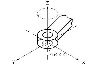
Depending on the required movement method, Matlab provides a number of building blocks to choose from for modeling them. In this work, the Revolute Joint block was used, which rotates the part about the Z axis in global coordinates (0; 0; 0), as shown in Figure 2.1.

Figure 2.1 – To an explanation of the Revolute Joint block
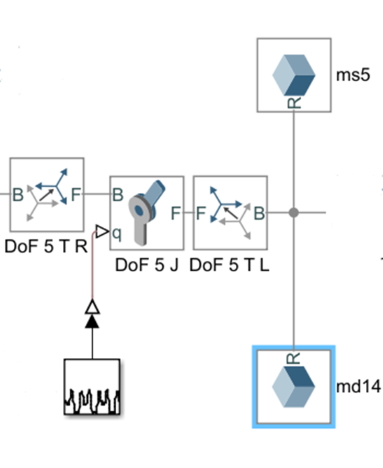
From the principle of operation of Revolute Joint: we bring the part to the required coordinates using the Rigid Transform block, then sequentially turn on the Revolute Joint block (DoF 5 T R in Fig.2.2), then, using the Rigid Transform block, return the part to its original position.

Figure 2.2 – Realization of movement of one joint
To evaluate the operation of the robot model, we used standard Simulink signals, which are fed through the Simulink–PS Converter block to the Revolute Joint input, having previously configured it for a given purpose. It is possible to set the law of changing the moment (Torque) and directly to the motion (Motion), it is also possible to remove the parameters automatically calculated in Matlab from this block. In this work, the law of motion (Motion – Provided by Input) is set, where the moment is calculated automatically.
The Revolute Joint block can also act as a sensor, taking readings of the angle of movement, angular velocity, acceleration from the joint, and also, which is useful in the design and development of movement algorithms, the moment required to make a given movement.
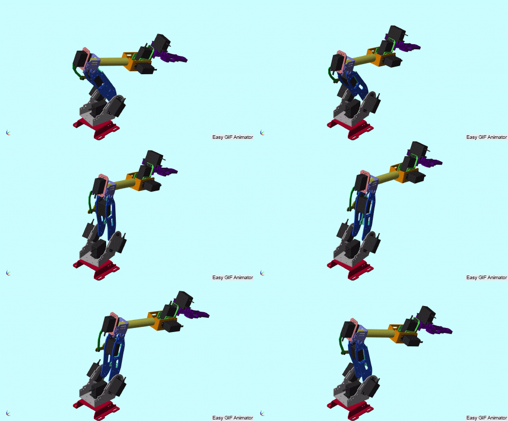
The resulting model can be used to estimate the movements of the robot.

Figure 2.3 – The result of modeling in the Matlab environment
(animation: 10 frames, 6 loops, 188 kilobytes)
3. Solution of the inverse kinematics problem
To control the movement of the end link of the manipulator (gripper), it is necessary to solve the forward and inverse problems of kinematics with a certain time interval. In contrast to the direct problem, the main problems are associated with the solution of the reverse one. The relevance of solving the inverse kinematics problem especially increases when manipulating manipulators with an excessive number of links in the mode of small time intervals. Currently, many methods have been developed that can solve the OZK for these manipulators, for which obtaining analytical solutions is not possible or rather difficult. Let's consider some of them. The method of inverse transformations simplifies obtaining a solution to the OZK, but does not solve the problem of unambiguous solution. The penalty function method, which uses solutions to nonlinear programming problems, and methods based on the properties of neural networks, require too much computation time, which makes them difficult to use in real time. The biquaternionic solution of the kinematic control problem, which reduces the solution to the Cauchy problem for the system of differential equations of kinetostatics, may not always have a solution. The method of intervals for solving the OZK is intended for simple kinematic schemes of manipulators.
4. Computer vision tools used to solve the sorting problem
Computer vision is a technology for creating machines that can detect, track, and classify objects. It uses statistical methods to process data, as well as models built using geometry, physics and learning theory. The main branch of computer vision is the extraction of information from an image or sequence of images. This is most often used to identify and recognize an object. Object recognition is divided into two stages: image filtering and filtering results analysis.
Edge detection is a term for a set of mathematical techniques designed to identify points in a digital image where the brightness of the image changes dramatically. These points are usually organized as a set of curved lines. Selected edges can be of two types: point-independent and point–of–view. Independent boundaries display properties such as surface color and shape. The contributors can change at different viewpoints and represent the geometry of the scene. One of the simplest and most natural ways of image binarization is brightness threshold transformation. Binarization — converting an image to monochrome. Typically, areas of the image that have been filtered are colored white, and the rest of the image is colored black.
Among the many methods of processing filtering results, several are distinguished: algorithms for contour analysis and algorithms for neural networks. Contour analysis allows you to describe and produce objects that are presented in the form of their external outlines – contours. The outline contains all the necessary information about the shape of the object. But the interior points of the object are not counted. This limits the way of applying contour analysis, but allows you to move from a two–dimensional space of images to a space of contours, which can greatly reduce the algorithmic and time complexity of the program.
Conclusions
This paper analyzes a method for implementing a prototype of a robot–sorter. Conclusions are drawn about its structural components, hardware and software are selected to solve the problem. A simulation model has been created for debugging control algorithms.
References
- Анучин А.С. Системы управления электроприводов/ Анучин А.С .: Издательский дом МЭИ, 2015. – 54 с.
- Raspberry Pi 4 Model B specifications [Электронный ресурс]. – Режим доступа: https://www.raspberrypi.org/....
- PCA9685 [Электронный ресурс]. – Режим доступа: https://micro-pi.ru/....
- OpenCV [Электронный ресурс]. – Режим доступа: https://opencv.org/about/.
- NumPy [Электронный ресурс]. – Режим доступа: https://numpy.org/.
- SciPy [Электронный ресурс]. – Режим доступа: https://www.scipy.org/.
- Adafruit CircuitPython [Электронный ресурс]. – Режим доступа: https://circuitpython.readthedocs.io/projects/servokit/en/latest/.
- Simulink. [Электронный ресурс]. – Режим доступа: https://matlab.ru/products/Simulink.
