Tushar S. Chande

Effects of Exits and Portfolio Strategies on Equity Curves

Раздел главы 6 книги Tushar S. Chande «Beyond Technical Analysis: How to Develop & Implement a Winning Trading System»

Источник: Коммерсант, деловая онлайн библиотека

All the decisions you make about entries, exits, and stops show up in the slope and smoothness of the equity curve. In this section we will explore the equity curves of the 65sma-3cc model using a deutsche mark actual contract with rollovers. We will study how the equity curve responds to changes in system design. Our yardstick for comparison will be the standard error calculations described in the previous section. We will not test continuous contracts, because the actual contracts with rollovers provide a better simulation. Besides, the System Writer Plus™ software from Omega Research can be used here to develop detailed equity curves.

The test set includes actual deutsche mark contracts from March 1988 through September 1995. We allowed $100 for slippage and commissions, and the software automatically rolled over the contracts on the 20th day of the month preceding expiration.

The procedure is as follows: the daily equity of the test case is exported into an ASCII file, which is then imported into the Microsoft Excel 5.0 spreadsheet. The regression calculations are perfomed in Excel using their built-in tools for regression analysis, as explained in the previous section.

We first tested the 65sma-3cc model on the deutsche mark contracts without any stops or exits (case 1). The case 1 equity curve (Figure 6.6), has a linear regression slope of $17.54, and a standard error of $4,043. During the test period, the 65sma-3cc model produced paper profits of $24,288, with a profit factor of 1.34 and a maximum intraday drawdown of -$11,938, trading one contract at time. The equity curve for case 1 is rather jagged, with a significant retracement in 1992, and is typical of trend-following systems without any exits. Note how many trades gave up significant profits before being closed. Also, if the market enters an extended sideways period, this model will suffer drawdowns, and you can go a long time before new equity highs.

Figure 6.6 Case 1, the 65sma-3cc model without any stops or exits, on actual deutsche mark data with rollovers

Case 2 is the same system with a $1,500 hard stop. The equity curve (Figure 6.7) shows that adding this stop decreased profits and reduced smoothness compared to case 1. The net paper profit dropped sharply from $24,288 to just $6,913, for a meager profit factor of 1.10. The maximum intraday drawdown almost doubled, to -$20,225, suggesting that a $1,500 stop is too tight. The equity curve (see Figure 6.7) shows the lower profit and higher drawdown. Note that the slope has halved from case 1, to $8.24, and the standard error has increased to $7,517. Hence, when you set your stop, compare the hard dollar amount to the market's volatility, and ensure you are safely outside its zone of random movements. Many traders seem to favor tight or close stops, and these calculations suggest that tight stops may degrade long term performance.

Figure 6.7 Case 2, the deutsche mark contracts and 65sma-3cc system with $1,500 initial stop

In case 3, the stop was increased to $5,000. This produced the same results as case 1. Thus, at $5,000 the initial stop was so wide that it produced results identical to testing without any stops. Thus, returning to the volatility argument, you should check that your stop is not so wide that it is virtually the same as not using a stop at all. Of course, a wide stop will act as firewall of last resort, and is useful for the occasional hiccup in the markets.

Many traders agree that exit strategies play a crucial role in a system's ultimate success. A common practice is to use several exits for a single entry signal. The 65sma-3cc system was tested with two exits, one an exit at the lowest low or highest high of 10 days, and the other the volatility-based exit discussed in chapter 5.

The result of using both these exits (case 4) with a $5,000 initial stop was to reduce the paper profits even further, to $3,737, for a paltry profit factor of 1.07. The maximum intraday drawdown of -$13,337 was actually larger than the calculations with no stops at all. You would expect the equity curve to be smoother as a result of the exits. As Figure 6.8 shows, the slope decreased to $5.08 and the SE was $3,368. The new slope was only 29 percent of the slope without stops, but standard error was only 17 percent smaller. Thus, there was a sevenfold drop (85 percent reduction) in reward for only a 17 percent reduction in risk – too high a price to pay for this system.

Figure 6.8 The 65sma-3cc system on DM with trailing stop, volatility stop, and $5,000 exit

Notice how the equity curve for case 4 looks qualitatively different from that for case 1, because it has "flat" portions where the exits take the system out of the market. Case 4 neatly illustrates one of the trade-offs in system design: you can go for higher profits or a smoother equity curve. Your choice may depend on many factors, including your personal preferences for risk and equity fluctuations.

We next consider a delayed 20-bar breakout system with a $5,000 initial stop and a trailing stop at the 14-day high or low (case 5). The DM contracts over the same period for this case yielded a slope of $8.36, with a SE = $1,960. Case 5 had a clipped equity curve (see Figure 6.9) with many flat portions when the model was out of the market. The equity shows that this approach successfully caught some of the trends, and avoided most of the sideways markets.

Figure 6.9 Equity curve for a delayed breakout model with $5,000 stop and 14-day high-low trailing stop

You must be careful not to judge the relative smoothness of an equity curve simply by inspecting it visually. For example, consider case 6, the equity curve obtained by adding those for case 1 and case 5. This equity curve (Figure 6.10) seems smoother to the eye than the equity curve for case 1. Besides, we are adding an equity curve to case 1 that has just half of its SE. A regression calculation shows that the slope of the joint equity curve is $25.90 and the SE = $5,263, bigger than either curve. You may find this easier to believe if you grasp that the profitable periods coincide, increasing the amplitude of the movement during these overlapping periods. The result is an equity curve with larger standard error. Thus, you should check the regression numbers when you combine multiple systems on the same market.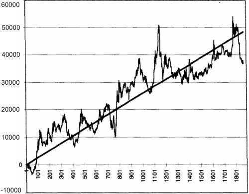

Figure 6.10 Case 6 combined equity curve for case 1 plus case 5

Note that due to its greater slope, the composite equity curve (case 6) has a higher reward/risk ratio (25.90/5263 = 0.00492) then the original case 1 (17.54/4043 = 0.00434). Thus, we could improve the risk/reward ratio by combining systems using different logic to trade the same market.

You should not underestimate the potential difficulties caused by positive covariance. Figure 6.11 shows the effect of combining two DM systems with positive covariance. The usual rules for combining variance of two independent systems predicted a standard error of $5,430. The actual calculated SE was $6,935, about 28 percent greater. The two systems have positive covariance because they tend to make (or lose) money at the same time, at least some of the time. Figure 6.11 shows lines one standard error on either side of the best fit line. These SE lines include most, but not all, of the points of the joint equity curves. The points that lie outside the SE bands occur when both systems "reinforce" each other, when they make money at the same time. Thus, combining systems with positive covariance will increase SE and reduce smoothness. Now add the complication that we do not know how covariances will change in the future. Therefore, improvements in smoothness may not result from simply adding different systems trading the same market.

Figure 6.11 Trading two systems on the DM market with strong positive covariance increases SE and equity curve roughness. The lines above and below the best fit line are one standard error away

One popular prescription for smoothing the equity curve is diversification through trading multiple markets. The equity curve for the cotton (CT) market, using the 65sma-3cc system from February 22, 1988, through June 20, 1995, with a $5,000 stop is shown in Figure 6.12. The system reported a profit of $28,720, with a profit factor of 1.64, and a maximum intraday drawdown of -$7,120. As usual, $100 was allowed for slippage and commissions in these calculations. Regression calculations showed a slope of 11.65 and a SE of $3,184. The 65sma-3cc calculations for DM for the same period and conditions as the CT calculations yielded profits of $24,900 with a profit factor of 1.34 and a maximum intraday drawdown of -$11,687.

Figure 6.12 Equity curve for CT using the 65sma-3cc system

The CT and DM equity curves to test for increased smoothness. The assumption here is that the CT and DM markets are not dependent on each other. The regression analysis of the joint CT plus DM equity curve (Figure 6.13) showed a slope of $29.34 and a SE of $5,265. The increase in slope is understandable, since adding the two markets roughly doubled the profits over the same period. The joint slope for CT and DM is the sum of their individual slopes ($29.34 = $11.65 + $17.69). The rules for combining variance suggest that if the two markets were independent, then their variances (squared standard error) would just add up linearly. This indicates that the expected value of the standard error for the joint CT + DM equity curve is $5,098. However, we see that the actual value is slightly higher, at $5,264, implying some positive covariance. Thus, we could not have reduced equity curve roughness by combining these two markets. We can show that adding more markets to a portfolio does not increase smoothness (reduce SE) unless the two markets are negatively correlated. Usually, there is some weak correlation between markets due to random or fundamental factors, and markets rarely move exactly opposite to each other. Hence, we should expect roughness (or SE) to increase as we combine the equity curves from different markets.

Figure 6.13 The joint CT + DM equity curve

In summary, the SE of the equity does not automatically decrease when you change exit strategies, combine different systems on the same markets, or combine different markets on the same system. However, changing entry strategies can change SE significantly. This conclusion goes a bit against the popular wisdom that "diversification" gives a smoother equity curve. Diversification in this context means trading many different markets with the same system, or the same market with many systems. Of course, we are measuring the smoothness using the standard error from linear regression analysis. We saw in the previous section that increasing the slope does not reduce the SE.

You should use the information in this section to understand how system design and portfolio strategies can affect the smoothness of your equity curve. In this section we examined the daily equity curve for individual markets or systems. In the next section we look at the monthly equity curve and how it changes with money-management rules.

наверх