Denis I. Okhrimenko

Faculty of Ecology and Chemical Technology
Department "Fuel Chemical Technology"
Specialty "Chemical technology of fuel and carbon materials"

Research supervisor: c.s.c., docent Vladimir V. Oshovskiy

Abstract

Contents

Introduction

       The most chemical engineering problems and even the problems of the engineering practice somehow are associated with fluid dynamics processes. A fluid dynamics processes are extended, but has a complex nature in theory as well as in the realization aspect.

The master's thesis purposes and the problems. The theme topicality

       The theme topicality. At the countries of the CIS the computational fluid dynamics (CFD) use practice was appeared comparatively not long ago and just only at the sectors which require high-accuracy calculations – aviation, aerospace industry. The use of CFD is allowed to decrease expenses and to increase a designing speed considerably. That is why, the implement question of it at the designing process is extremely topical problem.
       The master's thesis purpose is to use the numerical techniques of the engineering simulation software for receive the flow characteristics at the chemical engineering object. Also, is to compare the numerical results with measured data.

Topic review

       The docent George G. Pyatyshkin from the Department of the Industrial Heat-Power Engineering.
       The finite-element systems were used by Bolotin E.O., Voloshin V.V., the masters of the DonNTU, in their master's theses, to simulate the liquid flows and the gas flows of the industrial objects. Stetsenko V.Yu. used the finite-volume method in her master's thesis.
       In Ukraine the finite-element based software is used in general with the design institutes, infrequently with the research institutes.
       In the world such software is used with the design institutes as well as with the research institutes actively.

The some aspects of the fluid dynamics

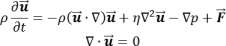
       Fluid dynamics governing equations is the Navier-Stokes equations. The system is consist of the momentum equations and the continuity equations [1,2,3].
       For the Incompressible Newtonian fluid the Navier-Stokes equations in their most general form read:

(1)

where η – the dynamic viscosity, Pa·s; ρ – the density, kg/m³; – the velocity vector, m/s; p – pressure, Pa; – the body force vector, N/m³; t – time, s.
       There are two flow types in the fluid dynamics – the laminar flow and the turbulent flow. Exactly turbulent flow gives rise to special difficulties for research and modeling. Turbulent modeling is one of the most difficult and unsolved problems of the fluid dynamics and the theoretical physics [4].
       Now, exist a lot of models for turbulence flows simulation. It differ one from another in computational complexity and in computational accuracy.
       In [5] was shown one of the most used and simple turbulence model – RNG (renormalization group) based k-ε model.
       Initial and boundary conditions. Initial and boundary conditions are needs to be formulated so as to system of equations (1) definitely characterize velocity and pressure distribution.
       The transient problems requires an initial distribution of the fluid velocity components, and it need to be obey the continuity equations [6].

The some aspects of the computational fluid dynamics

       The basic CFD problem is the numerical calculation of the Navier-Stokes equations describes the flow dynamics. In addition is taken account of different physicochemical effects: combusting, turbulence or flows through the porous medium [7].
       Numerical calculations can be carry out only when the governing principles are expressed in mathematical form, usually in form of differential equations [8]. The Navier-Stokes equations include the linear differential operators and also nonlinear differential operators, so they are interesting [9].
       The main idea of the numerical calculation is a differential equations approximation – a discrete analog construction. As a result, the problem solving turns into the system of linear algebraic equations.
       Now the finite-element method and the finite-volume method have a greatest abundance.
       Finite-volume method. The main idea of the finite-volume method (FVM) is next. The calculation domain is divided into the some noncrossing control volumes. The differential equation is integrated by each control volume. To calculate the integrals the piecewise polynomial function is used, which describes a change of the unknown function between the reseau points. As a result the discrete analog is constructed, which consists of the unknown function values in several reseau points.
       Finite-element method. At the finite-element method (FEM) the calculation domain is divided on the triangular and quadrilateral elements. Usually, a discrete analog is received using variational principle, if it exist, or using Galerkin method. An assumptions of the shape function is used to describe the dependent variable behavior on the element [8].

An engineering simulation software based on the CFD

       The widespread simulation software based on the CFD are: ANSYS, COMSOL Multiphysics, CFdesign, FlowVision, Star-CD and others.
       For the creation and calculation of any problem the next sequence of operations is recommended:

1. Choose the space dimension, define the physics chapter and define transient or steady-state analysis.
2. Define the workspace and specify a geometry.
3. Specify the variables.
4. Assign the physical properties and initial values.
5. Assign the boundary conditions (BC).
6. Grid Generation.
7. Assign the parameters of the solver and solve the problem.
8. Get a results [10].

       The velocity field and pressures calculated using FEM during constriction flowmeter simulasion is shown in Figures 1 and 2. Flowmeter general properties:

	Fluid		water;
	Fluid temperature		20°С;
	Tube diameter		D = 0,03 m;
	Flowmeter aperture diameter		d0 = 0,024 m;
	Flowmeter thickness		δ = 0,002 m;
	Pressure loss (flow average velocity 1.4 m/s)		900 Pа.

       Equations: standard k-ε turbulence model.
       Boundary conditions:

	- Inlet:		Poiseuille parabolic profile with maximum of 1 m/s; Turbulence intensity – 0.05; Turbulence length scale – 0.07D (D – cross-section diameter)
	- Outlet:		Pressure – 101325 Pа
	- Wall:		Logarithmic wall function. Wall offset – h/2 (h – mesh element size)

       Mesh consist of 7039 triangular elements and 4019 mesh points.

Fig. 1. Velocity field	Fig. 2. Relative pressure

       The results of the transient analysis modeled using FVM is shown below. (Fig. 3 and Fig. 4)

Fig. 3. Velocity oscillation (30 frames, 7 repeats, 40 ms delay)	Fig. 4. Pressure oscillation (30 frames, 7 repeats, 30 ms delay)

The experimental procedure

       The experimental procedure consist of building the experimental model, carry out an experiment with registration the main characteristics. Numerical simulation. Comparing calculated results with measured data. In case the model adequacy carry out an optimization within numerical experiment. At the end, carry out an experiment using optimized parameters.
       It should be noted that this stage of the master's thesis is designing now.

Conclusions

       The CFD is the universal tool for process analysis of the fluid flow, heat transfer and mass transport. The purpose achievement will be allowed to validate numerical experiment adequacy for the umpteenth time; also, it will be allowed to research the hydrodynamic flow pattern of the research object and to optimize it’s parameters.

References

1. Касаткин А.Г. Основные процессы и аппараты химической технологии. – М., 1970. – 784 с.
2. Дытнерский Ю.И. Процессы и аппараты химической технологии: Учебник для вузов. Изд. 2-е. В 2-х кн.: Часть 1. Теоретические основы процессов химической технологии. Гидромеханические и тепловые процессы и аппараты. – М.: Химия,1995. – 400 с.: ил.
3. Гельперин Н.И. Основные процессы и аппараты химической технологии. – М.: Химия, 1981. – 812 с.: ил.
4. Ошовский В.В., Охрименко Д.И., Сысоев А.Ю. Использование компьютерных систем конечно-элементного анализа для моделирования гидродинамических процессов // Наукові праці ДонНТУ. Cepія: Хімія i хімічна технологія, 2010. – Вип. 15(163). – С. 163-173.
5. Черный С.Г., Шашкин П.А., Грязин Ю.А. Численное моделирование пространственных турбулентных течений несжимаемой жидкости на основе k-ε моделей. // Вычислительные технологии, 1999. – Том 4, №2. – С. 74-94.
6. Кутепов А.М., Полянин А.Д., Запрянов З.Д., Вязьмин А.В., Казенин Д.А. Химическая гидродинамика: Справочное пособие. – М.: Квантум, 1996. – 336 с.
7. Система моделирования движения жидкости и газа FlowVision. Версия 2.05.04. Руководство пользоватея. – М., 1999-2008. – 310 с.
8. Патанкар С. Численные методы решения задач теплообмена и динамики жидкости: Пер. с. англ. – М.: Энергоатомиздат, 1984. – 152 с., ил.
9. Фирсов Д.К. Метод контрольного объема на неструктурированной сетке в вычислительной механике. Уч. пособие: – Томск, 2007. – 72 с.
10. Егоров В.И. Применение ЭВМ для решения задач теплопроводности. Учебное пособие. – СПб: СПб ГУ ИТМО, 2006. – 77 с.