Content
- Introduction
- 1. Theme urgency
- 2. Methods of forecasting financial markets, based on the multiplicative model
- Conclusions
- The list of sources used
Introduction
Financial markets last ten years in a period of rapid development and globalization of communications. Along with the major national stock, futures, foreign exchange markets, the markets have appeared worldwide, is a typical representative of a modern financial market FOREX.
FOREX is a global network of banks, investment funds and brokerage houses, which includes computer infrastructure, serving clients who trade currencies and to profit from changes in foreign exchange speculation engaged. Daily turnover on the FOREX market exceeds one trillion dollars, according to the experts will continue to grow.
It is known that about 99% of all transactions in financial markets–speculative, are solely for the purpose of obtaining profits from the scheme buy cheaper – sell higher price
. All are based on forecasts of changes in quotations by market participants. To effectively analyze the market needs corresponding to modern requirements of economic and mathematical methods. Today a huge amount of scientific work in developing methods of forecasting the financial markets. Thus, research on stock markets – current and future activity and will remain so for quite some time.
1. Theme urgency
Anticipation – a prediction of future events. The aim of forecasting is to reduce the risk when making decisions. Weather is usually obtained in error, but the error depends on the predictive system. By providing a forecast of more resources, you can increase the prediction accuracy and reduce the losses associated with the uncertainty in decision making.
Forecasting economic and financial time series is an extremely urgent task. Current approaches to this problem can be characterized by the following areas:
1) approximation of the time series and extrapolation of analytic functions found in the direction of the future – the so-called trend model [1];
2) study the effect of all possible factors in the figure, which is projected and the construction of econometric, or more complex models using group method of data handling (GMDH) [2];
3) modeling of future prices as a result of decision-making with neural networks, genetic algorithms, fuzzy sets [3]. Unfortunately, these techniques do not demonstrate a stable outlook, which could be explained by the complexity of systems whose dynamics are projected to permanent changes in their structure [4].
2. Methods of forecasting financial markets, based on the multiplicative model
The investigated time series is the result of a process. The most common method for studying the cyclic process is the classical seasonal decomposition. It is based on the possibility of providing time-series data in two models - additive and multiplicative. In these models, there are three components:
1) The trend reflects a long-term changes that occur in the time when the cyclical and irregular components removed.
2) Inflation reflects variations in the time series due to certain factors. Cyclical factor, usually repeated over a period, though the exact picture of the number of parameters can vary.
3) The random component - is the impact that may occur after excluding the influence of trend and cyclical factors.
To describe the dependence of the studied range was proposed by the classical regression model that takes into account two main components of time series - the trend and cyclical component. It has the form:
Yi=a0+a1Xi*cos(a3Xi+a4)
We assume that the quality of the forecast depends on the size of the window – the amount of data on which the relationship will be built, and the displacement of the window relative to the first element. Forecast is calculated on the next unit of time. The quality of the forecast estimated the multiplicative error.
The calculations were carried out in the software package Maple 15. In the calculations we used the following indicators:
p1 – the ratio of the actual value to the estimated time series;
m – the size of the window of time;
sdv – the offset time window relative to the first element.
As the study data, the values of the FOREX market quotations for November 2011. The analysis was performed according to intervals of different length of time and offset time window relative to the first element.

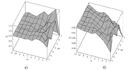
Figure 1 – The dependence of the quality of the forecast from the window of time
(a – taking into account the full dependence of the model parameters,
b – the phased identification of dependencies).
Figure 1.a shows the dependence of the quality of the forecast from the window of time in the 10 units in the analysis of the FOREX market with an interval of time a day. In the calculation program takes into account the full dependence and calculated once all the parameters of the model. The optimal values of the ratio stands at one. Thus, the value of p = 1.05 at m = 2 sdv = 3 is the best.

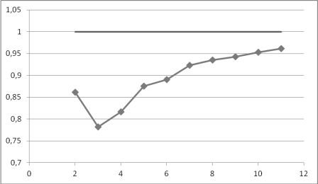
Figure 2 – The dependence of the quality of the forecast of the size of time window.
Figure 2 shows the change in value of the average values of the ratio of the actual value to the estimated time series for the examined period of time. Thus, with increasing window size increases the quality of the forecast. From the calculations show that the difference from best to worst prediction accuracy is 22.4%.
Analysis of the dependence of the second method (figure 1.b) took place in two stages: at first turned out to be a trend, then took away from the source data value of the modeled trend, and the residue was found a circular dependency. The optimal value of the ratio of the window size and offset relative to the first element is the value of p = 0.92 at m = 10, sdv = 3.

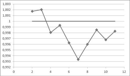
Figure 3 – The dependence of the quality of the forecast of the size of time window.
Change the value of the average values of the ratio of the actual value to the estimated time series for the investigated period of time with the second method of calculation is shown in Figure 3. The highest prediction accuracy is observed in the time window 5 points. The difference the best and the worst prediction accuracy is 3.4%, indicating that the greater reliability of the method.
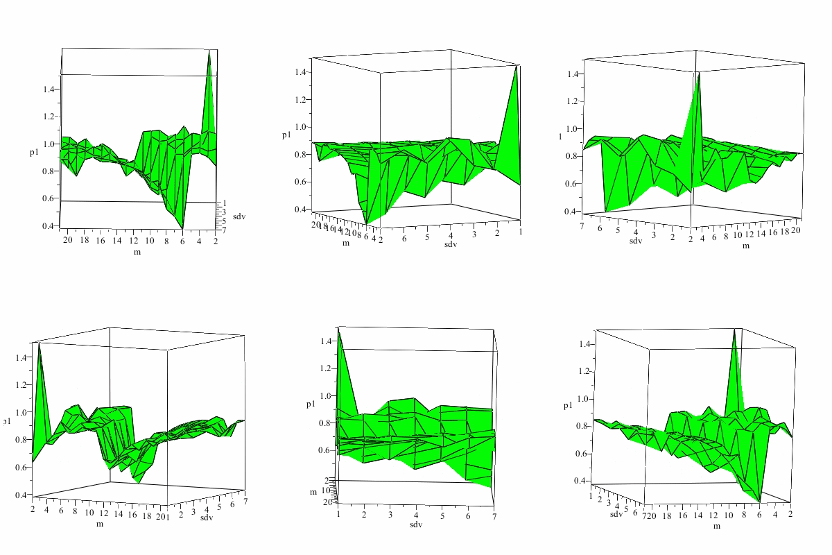
Figure 4 shows the dependence of the quality of the forecast from the window of time in the 20 units in the analysis of the FOREX market with an interval of time 1 hour.

Figure 4 – The dependence of the quality of the forecast from the window of time 20
(animation: frame rate - 17; size - 400x400; delay between shots - 50 ms; number of cycles of repetition - 3; volume - 286 KB).
Conclusions
The principle of hierarchy of temporal increments allows maximum use of the information contained in the time series to construct the forecast. The outlook on technology complex Markov chains in the range of standard deviations and the distribution is close to the modal values, which means that this method gives an estimate of the accuracy of the method of complex Markov chains.
In this paper we present an analysis of the FOREX market quotes values for November 2011 with an interval of a different period of time and offset time window relative to the first element. It was determined that the most accurate prediction is achieved by the second method to identify a trend, but the optimal values are achieved, taking into account the full dependence of the model parameters by the first method. The results obtained are local for the given time interval in a certain stability.
Future work will apply sophisticated technology Markov chains for financial time series prediction with a comparative analysis of the results [4,5].
In writing this essay master's work is not yet complete. Date of Final Completion: December 2012.
The list of sources used
- Принципи моделювання та прогнозування в екології. / Богобоящий В.В., Курбанов К.Р., Палій П.Б., Шмандій В.М.– К.: Центр навчальної літератури, 2004. – 216 с.
- Зайченко Ю. П. Нечеткие модели и методы в интелектуальных системах: учеб. пособие для иностр. студ. вузов, направления "Компьютерные науки" / Зайченко Ю. П.,М.З. Згуровский. – К.: Слово, 2008. — 344 с.
- Ежов А.А., Шумский С.А. Нейрокомпьютинг и его применения в экономике и бизнесе. – М., 1998.
- Чабаненко Д.М. Алгоритм прогнозування фінансових часових рядів на основі складних ланцюгів // Вісник Черкаського університету. – 2010. – Вип 173. – С. 90-102.
- Prediction of financial time series with hidden markov models/ Yingjian Zhang, Simon Fraser University, 2004.
- Сорос Дж. Алхимия финансов/ Пер. с англ. Аристова Т.С. – М.: ИНФРА–М, 1999. – 416 с.
- Курбанов К.Р., Сапцин В.М. Сложные цепи Маркова как технология прогнозирования социальных, экономических и экологических процессов. // МНПК аспір., мол. учених та науковців. «Проблеми та перспективи розвитку регіональної ринкової економіки» Кременчук, 11-13 травня 2007 р. С. 10-14.
- Сапцин В.М. Опыт применения генетически сложных цепей Маркова для нейросетевой технологии прогнозирования. Вісник Криворізького економічного інституту. – Кривий Ріг: КЕІ КНЕУ, 2009. – Вип. 2 (18). – С. 56–66.
- Соловйов В.М. Математична економіка. [Навчально-методичний посібник для самостійного вивчення дисципліни] / Соловйов В.М. – Черкаси: ЧНУ, 2008. – 136 с.
- Prediction of financial time series with the technology of high-order Markov chains [електронний ресурс] / Soloviev V., Saptsin V., Chabanenko D. // Working Group on Physics of Socioeconomic Systems (AGSOE). – Drezden , 2009. – Режим доступа: http://www.dpg-verhandlungen.de/ 2009/dresden/agsoe.pdf
- Романовский В.И. Дискретные цепи Маркова / В.И. Романовский. – М.-Л.: Гостехиздат, 1949.
- Zhang Y. Prediction of Financial Time Series with Hidden Markov Models / Y. Zhang // School of Computer Science. – Vol. Master of Applied Science: Simon Fraser University, 2004.
- Rabiner L.R. A tutorial on hidden markov models and selected applications in speech recognition / L.R. Rabiner // In Proceedings of IEEE. – 1989. – Vol. 77. – P. 257-286.
