
Abstract
- Introduction
- 1. Relevant topics
- 2. Purpose and objectives of the research
- 3. Overview of Research and Development
- 4. Current outcome
- Conclusion
- List of sources
Introduction
Currently thermometer anemometers are
widely used to measure various
physical and chemical parameters of the gas streams. In particular, the
TA is
successfully used to control the speed and expenditure of ventilation
flows in
constructions of various architectural buildings and in the course of
their
operation, to conduct research works to study the dynamic parameters of
turbulent flows, and for measuring the concentration of explosive gases
in the
automotive industry for the optimization of internal combustion
gasoline
engines , in the study and control gas stream flow-around of compound
bodies,
and for gas flow measurement in large pipes, etc. [4].
1. Relevance of the topic
Today is a very urgent task to develop
technical means
for the experimental determination of the dynamic characteristics of
speed
measuring devices and temperature gas streams. At the Donetsk National
Technical University department of electronic engineering jointly with
the Donetsk
National University Technological
Bureau
"Turbulence" begun works of
creation corresponding test
equipment in the form of a specialized number of aerodynamic of stands.
In this
regard, there is a need to develop fine structure of turbulence classic
measuring device to perform works on the metrological certification of
developed stands.
Analysis showed, that one of
the few
devices satisfy the requirements set, imposed to the means of measuring
the characteristics
of of turbulent currents, is the hot-wire anemometer
(hereinafter – the
TA) of.
The TA
Sensor substantially does not
disturb the flow, has a high spatial resolution for measuring the
microscale of
turbulence and low inertia while measuring pulsation [9].
2. The purpose and objecties of the research
The aim is to develop and study hot-wire
TA for measurement the fine
structure of turbulent gas flows in specialized aerodynamic stands. To
achieve
this goal following tasks are formulated in this work:
1. Overview the
methods and means of measurements of the local velocity and temperature
of the
gas stream;
2. Development of constant
temperature hot-wire anemometer to study the fine structure of
turbulent gas
flows;
3. Static calibration
of hot-wire anemometer and refinement of the heat balance equation;
4. Evaluation of
dynamic characteristics of the anemometer;
5. Justification of
the structural design of the electrical anemometer signal recording
system;
6. Use the method of three superheatings to separate signals of velocity and temperature.
3. Overview of Research and Development
In 1996 in
Russia was established Research and Production Association
"Turbulence-DON". It specializes in design and manufacture of
commercial facilities for gas, liquid, thermal power, telemetry
systems, and
also carries out metrological service of flow meters, a wide range of
services
for the design and construction of accounting systems energy resources.
By the
volume of the products the company is a leader in the country.
LLC SPA
"Turbulence-DON" – develops and manufactures such metering
devices:
stationary and portable gas hot-wire flow meters, municipal gas meters,
gas jet
flow; stationary and portable liquid flow meters (including sewage)
systems for
Heat; telemetry systems, pressure sensors, testing equipment, and also
provides
a wide range of services for calibration, maintenance, repair, testing
of all
types of gas flow meters [6].
In Ukraine, it
is necessary to determine the dynamic thermal performance of air flow
to solve
a wide range of practical problems in industry, environment, health and
safety.
This parameter control of HVAC systems, the microclimate in residential
and
industrial buildings, cabins and saloons vehicles, fume collection
channels and
pipes.
The
instruments used for these measurements
should have a wide range, both the velocity (from tenths to tens of
meters per
second) and the temperature (from tenths to several hundred degrees), a
high
sensitivity at low pressure differentials (unit Pascal). They must be
reliable
and easy to use, provide an indication of the measured parameter in
units of
physical quantities. These requirements are fully satisfy modern hot
wires.
In the Special
Design and Technological Bureau "Turbulence", in Donetsk National
University, developed and produced several versions of such hot-wire
devices:
- Thermoanemometer AIST-5. Autonomous
measuring
instrument of air flow velocity and temperature.
- Thermoanemometer IRIT-4. Flow
indicator and
traction.
- Thermoanemometer ISRV-2.Thermoanemometric gas meter [2].
At the local level, in Donetsk National Technical University similar issues related to the development of hot-wire anemometers for determination of the fine structure of turbulent gas flows were studied by such masters as Chujko V. A., Morozov A.A., Czibulka V.S., Tymoshenko I.N.
4. Сurrent outcome
The concept of turbulent and laminar
flow was
introduced in 1883 by the English physicist O. Reynolds, studying the
motion of
the fluid in the pipe. At low speeds the movement is regular, but the
ratio of
inertial forces to viscous forces (Reynolds number Re = ud/v,
where u
– characteristic velocity, d – characteristic dimension of flow, in
this
case
diameter of the tube, v – kinematic viscosity) exceeds a critical
value
(ReK
= 103), the movement becomes stable and more
or less random. Thus in the
flow
appear irregular whirls of different sizes, and flow rate at each point
varies
randomly with time. These vortices can be crushed or sometimes merge
together.
The more so-called supercritical, i.e. the more Re excides ReK, the
more
intensive are the processes [7].
To observe the turbulence directly , we should make recognizable movement of the flow of water or air. In the air, it is easy to implement using smoke. On the figure 1 it is shown the turbulent motion of the gas [8].
Figure 1 – Animation of the turbulent motion of the gas (the number of frames - 7, volume - 142 KB, the number of cycles of repetition - 6 times, the delay between shots - 100 ms, the delay between repetitions - 200 ms)
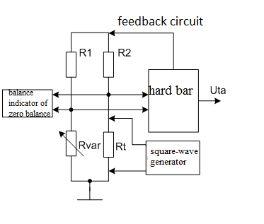
Figure 2 – Functional diagram of the developed hot-wire TA of the constant temperatur
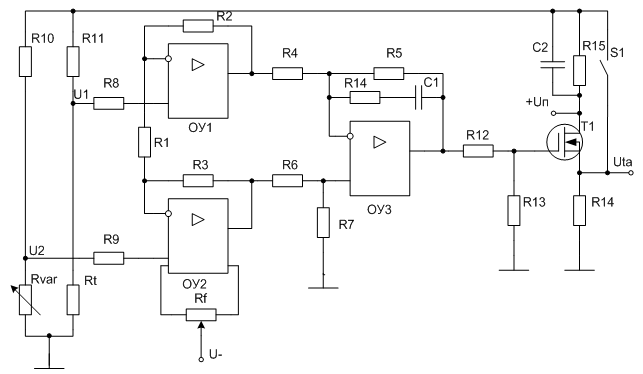
Figure 3 – Functional diagram of the developed hot-wire TA of the constant temperatur
Measuring bridge TA is built
according to the classical scheme. Wire sensor Rt of thermometer
anemometer is
joined into one of the arms. Sensing element is made of tungsten wire
of a
diameter in 8 microns. The thread is welded to holders located at a
distance of
4.5 mm by spot welding to provide a reliable electrical contact and
mechanical
connection strength. The sensor is fixed on a tool box that provides
rigidity.
To balance the zero bridge
and to overheat
the sensor on the stage of experimental studies used a resistance
multiplier Rvar. After choosing the
optimum value of the resistance it should be replaced by a fixed
resistor. The
ratio of Rt and Rvar arms is 1:10. In-feed of
the measuring bridge is made
by a constant current.
The hard bar of TA is made
according to
the scheme of the measuring amplifier on three operational amplifiers
(hereinafter – the OC). This circuit solution allowed
to gain a high
amplification factor, high input impedance and good
common-mode rejection
[3].
In case of equality R7/R6 = R5/R4 the output voltage of the
amplifier is
given:
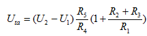 ,
(1)
,
(1)
The
use of discrete CO made possible to
select passive components for optimal parameters of the scheme. In
particular,
implemented the possibility of device frequency
compensation.
A distinctive feature of the
TA is using a field transistor FET IRF840 with insulated gate in the
feedback
circuit that has a low drain-source resistance in the ON state (0.850
ohm) and
fast switching time (21-35 ns), which improved the frequency response
of the TA
as a whole.
Methods of TA initial setup. During TA initial setup the following
operations must
be done:
1)
To enter the setup mode S1 is converted
into the open
state opening the feedback loop. In this case, the measuring bridge is
powered
by direct current through the resistor R15.
2) Produce Zero Balance of the
measuring bridge with a resistance box Rvar and dial gauge balance.
3) Determine the resistance of the "cold"
leg at room temperature according to the formula:
Rt=Rvar/10.
(2)
4) Switch
the TA to work, closing the key S1.
5) Preset the value
of overheating by using the
tungsten temperature coefficient of resistance (TCR) and the resistance
of the
string sensor at a certain ambient temperature.
6) Perform the
correction of the frequency response of
the TA. To do this the built-in square-wave generator is used, made on
a
microcontroller ATiny2313, deliver on the test input sensor in the form
of a
square waves with a frequency of about 2 kHz and a duty cycle of 2 [4].
Potentiometer Rf regulate the time constant of the instrument. The
optimum
setting when the peaks of the output signals are the most acute, but
disruption
of generation is not observed yet.
Achieved
by
means of field tests results allowed us to estimate the electrical time
constant of the measuring circuit TA, which was about 20 microseconds,
that
ensures the required bandwidth from 0 to 20 kHz.
Static calibration of
the TA
was
carried out in an aerodynamic stand ADS-200/250 with specialized
information-measuring system calibration of hot-wire sensors [3].
Calibration
was carried out in air flow velocity range from 1.5 to 10 m / s at
temperatures
from 20 to 45 0С. To enhance the reliability of
measurement results for
calibration was performed for three identical filar sensors
(hereinafter –
sensors number 1 – № 3) at three different filament
overheating: Tw =
100, 140
and 180 0С.
The experiment for each sensor were determined according to the output voltage of TA from the flow velocity at four temperatures: Tg = 23, 30, 38 and 45 0С. (see Fig. 4).
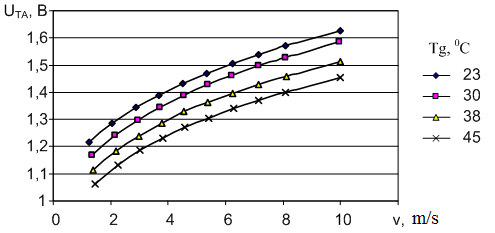
Figure 4 – A set of characteristic curves of TA output voltage from the flow velocity at different temperatures
The obtained results allowed to
determine the ranges
of output voltage of the TA and sensitivity of the speed at different
temperatures strands (see Table 1). Based on the analysis of the
results the
requirements for the analog-to-digital converter (ADC) signal
processing
circuit TA are made:
- Operating voltage range from 0 to 2.5
V;
- Capacity to determine the static
characteristics –
at least 10;
- Capacity to determine the dynamic
characteristics –
at least 12.
Table 1 – The output range of the TA voltage and sensitivity over the speed at the minimum and maximum temperature thread overheating
|
Filament temperature Tw, 0С |
Output voltage ТА
UТА, |
Sensitivity velocities S, В·с/м |
|
100 |
1,05..1,65 |
0,03..0,085 |
|
180 |
1,55..2,25 |
0,08..0,125 |
Elaboration of the heat
balance equation TA. As a basic heat balance equation for
the approximation of obtained in the
calibration of the experimental measurement data was chosen recommended
in [5],
the expression of the form
P / (Tw – Tg) =
(A + B(ρv)n)
· (Tw / Tg)m,
(3)
where P – power supplied to the SE, W;
Tw, Tg – SE
temperature and flow respectively, K; ρυ – mass
flow rate, kg/(m2*s); A, B, n
and m – constants coefficients determined by
individual
calibration of
the
sensor.
While sensor calibration data processing
and analyzing
as the result of solving non-linear regression calibration coefficients
was
found that temperature correction power function
included into the basic equation (3) did not
accurately describe the temperature dependence of the coefficients A
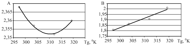
and B. Figure 5 shows the typical form of the
dependence of the coefficients A and B
from the flow temperature Tg. It is specified that the coefficient A
the
experimental temperature dependence is well approximated by a quadratic
function of the form
A(Tg) = a2Tg2
+ a1Tg
+ a0
and for the coefficient V – linear
function
B(Tg)=b1Tg+b0
Thus, improved heat balance equation
takes the form
P / (Tw – Tg) = A(Tg) + B(Tg) · (ρv)n. (7)
а) б)
a) A (Tg); b) B (Tg)
The proposed
method of calculating the calibration coefficients for the improved
equation
(7) is as follows:
1) For the base equation (3) determine
the value of
the coefficient n.
2) At a fixed ratio of n = const
determine the values
of the coefficients Ai and Bi of corresponding i-th stream
temperature (i = 1
.. 4).
3) Approximates the dependence of B (Tg)
function (6).
4) Clarify the meaning of Ai and
approximate the
dependence of A (Tg) function (5).
5) Estimate approximation errors of
calibration
experimental data according to specified equation (7).
For the evaluation of the calibration
approximation
error was selected relative standard deviation (SD).
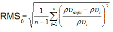 ,
(8)
,
(8)
where n – is the number of calibration points;
ρυ apr
and ρυ – the mass velocity, respectively found
in
the approximation and
experimentally.
The calculation results of errors in the calibration while using fundamental and improved heat balance equations are summarized in Table 2 and graphically presented in Figure 6. From the results it follows that in all the cases for different sensors and different superheating improved TA thermal balance equation (7) provides calibration error reduction in comparison with fundamental equation (3) at an average 1.7 times.
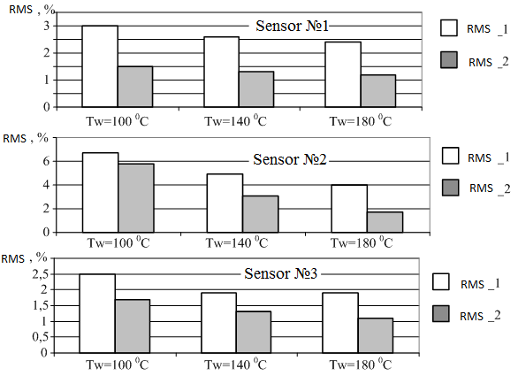
Figure6 – RMS approximation of the experimental calibration data fundamental (3) and improved equations (7)
Table 2 –Results of calculation errors of calibration by using a simple and improved heat balance equations
|
|
Sensor
№1 |
Sensor
№2 |
Sensor
№3 |
|||
|
Tw,0С |
RMS_1,% |
RMS_2, |
RMS_1,% |
RMS_2,% |
RMS_1,% |
RMS_2,% |
|
100 |
3 |
1,5 |
6,7 |
5,8 |
2,5 |
1,7 |
|
140 |
2,6 |
1,3 |
4,9 |
3,1 |
1,9 |
1,3 |
|
180 |
2,4 |
1,2 |
4 |
1,7 |
1,9 |
1,1 |
Conclusion
In
the
course of the work it was found that the electrical time constant of
the
measuring system ,developed by the anemometer, is 20 microseconds, that
provides the required bandwidth to 20 kHz obligatory for studies of the
fine
structure of turbulent flows.
Based on the
experimental results of the calibration the main metrological
characteristics
of the hot-wire anemometer identified and the requirements to the ADC
signal
processing are represented.
Taking
into
account the temperature dependence of the coefficients A and B, the
proposed
refined heat anemometer balance equation provided the increase in the
accuracy
of the calibration approximately into 1.7 times.
List of results
- Брэдшоу
П. Введение в
турбулентность и ее измерение – Москва, 1974. – 278
с.
- ДонНУ СКТБ «Турбулентность» [Электронный ресурс]. – Режим доступа: http://turbulence.uaprom.net/
- Зори А.А.,
Кузнецов Д.Н. Методы и программно-аппаратные средства
автоматизированной
системы градуировки первичных измерительных преобразователей
термоанемометров.
Известия ТРТУ.
Тематический выпуск: Материалы Всероссийской
научно-технической
конференции с международным участием «Компьютерные технологии в
инженерной
и управленч. деятельности». Таганрог: ТРТУ.
– 2002.
– №2 (25). –
С.148-150.
- Кузнецов Д.Н., Зори А.А., Кочин А.Е. Измерительные микропроцессорные системы скорости и температуры потоков газа и жидкости – Донецк: ГВУЗ «ДонНТУ», 2012. – 226 с.: ил. 125, табл. 16, библиогр. 95.
- Раннев
Г.Г.
Информационно-измерительная техника и электроника.
–
М.: Академия, 2006.– 512 с.
- Турбулентность
– Дон [Электронный
ресурс]. – Режим доступа: http://turbo-don.ru/
- Турбулентность [Электронный ресурс]. – Режим доступа: http://www.astronet.ru/db/msg/1188737
- Турбулентность
в потоке
жидкости или газа [Электронный ресурс].
– Режим доступа: http://www.physel.ru/mainmenu-4/eainmenu-15/198-s-193---.html
- Ярин Л. П., Генкин А. Л., Кукес В. И. Термоанемометрия газовых потоков. – Л.: Машиностроение, 1983. – 198 с.
- Повх
И.Л.
Техническая гидромеханика. 2-е изд., доп. / И.Л. Повх. –
Л.:
Машиностроение,
1976. – 504 с.