Abstract
Jian Ding and George Sperling. A gain-control theory of binocular combination.
This paper presents an artificial neural network for the adjustment of two cameras in order to picture the same spot for means of stereoscopic vision. The two cameras are in a master-slave relationship, where the optical center of the slave camera is adjusted to picture the same point as the optical center of the master camera. The task is performed by a biologically inspired five-layer artificial neural network with a complex structure and simple components. The network compares symbolic features of pixel surroundings on both images to determine the direction the cameras have to be driven into. The proposed system embedded in a neural hardware yields a robust and real time solution for camera control in stereo vision.
1 Introduction
Stereo vision is a process which recovers depth information about the scenes pictured by two or more cameras. It can be used in a vast variety of applications where spatial information about the objects is necessary. The proposed system is providing a control signal to two cameras to adjust their optical centers towards the point of interest making stereo vision possible. The system uses an Artificial Neural Network (ANN) to determine which direction the cameras have to be rotated. The control signal consists of two analog outputs, one for rotating to the right and the other for rotating to the left. The camera will turn to the direction represented by the higher output value.
The use of ANN in disparity matching to determine the 3D position of a point P is not a novelty. A neural network has already been used to compute the degree of matching between two pixels located on two different images in stereo vision. [3] In that case, an ANN was embedded in a program cycle which calculated the degree of matching for all the points under investigation. After the cycle was done, the left pixel and the right pixel with the highest matching degree were considered as the appropriate pixel pair.
The novelty of this paper is to present a neural structure to solve the problem presented above. The proposed structure does not necessitate the use of conventional computational tools, such as a Neuman based computer architecture. The program cycles are replaced with a vast ANN, where all the calculations are done in a parallel way. In addition, the network is constructed of neurons performing very simple tasks, such as additions, subtractions, etc. For this reason the input weights and the features of the transfer functions can be pre-determined, thus no learning is needed.
This paper is part of a research program whose aim is the modelling of the mental structure of a living creature. In our research the selected animal is the paradise fish (Macropodus opercularis) and its action–reaction movement habit is simulated. The key element of the system is the cognitive map that stores all the information about the living environment of the animal[8]. The vision system is the input of the system, it provides the learning and adaptation properties. The goal of the programme is to use biologically inspired technologies, for this reason the proposed matching system is based solely on an ANN.
The organization of this paper is as follows. In Section 2 we give a background about the theories used in the development of the proposed system. In Section 3 the proposed system will be described including the matching of pixel pairs, the proposed neural based system and the pre-adjustment of input weights and transfer functions. In Section 4 test results are presented, and finally in section 5 we conclude with a discussion of the results and we present the directions of further developments.
2 Background
Stereo imaging or stereo vision [1][5][6] refers to a process which transforms the information of two plane images into a 3D description of the scene and recovers depth information in terms of the exact distance. The basic idea of stereo vision is illustrated on Fig. 1.
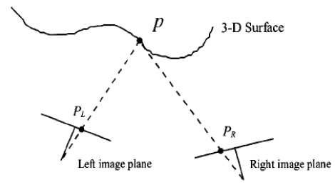
Figure 1: The basic concept of stereo vision
An arbitrary point in a 3-D scene is projected onto different locations in stereo images. Assume that a point p in a surface is projected onto two cameras’ image planes, PL and PR, respectively. When the imaging geometry is known, the disparity between these two locations provides an estimate of the corresponding 3-D position. Specifically, the location of p can be calculated from the known information, PL and PR, and the internal and external parameters of these two cameras, such as the focal lengths and positions of two cameras [2].
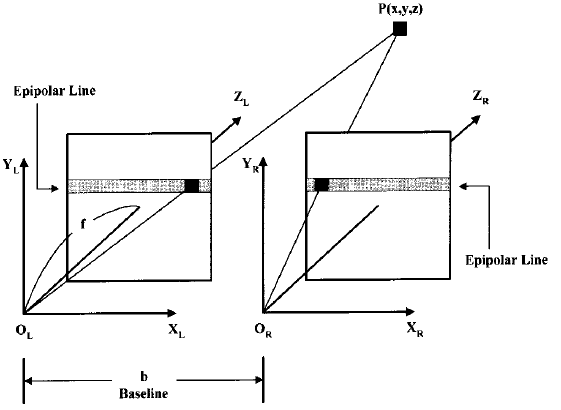
Figure 2: The parallel configuration in stereo vision
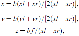
Shown in Fig.2 is a parallel configuration, where one point, p(x;y; z), is projected onto the left and right imaging planes at PL(xl,yl) and PR(xr,yr), respectively. The coordinates of p can be calculated as follows:
where (xl - xr) = the disparity, base line b = the distance between the left and right cameras, and f = the focal length of the camera. Thus if the disparity with respect to the two image planes of the point P is known, its spacial position can be calculated.

Figure 3: This is how the human eye can see a landscape
If we suppose to have a camera which provides a sharp image only in the center of the field of view, it is desirable do adjust the cameras into a position and orientation so that the point of interest P comes to the center of both image planes. This is where human vision comes into the scope. When the human vision system builds up a model of the surrounding world using the brain and the eye, it has to get visual information from the whole field of view. For this, the eyes have to scan the field of view with their optical centers adjusted to the point of interest. The reason is that in the retina there are rods sensitive to light and motion, and cones sensitive to color. For this reason the retina has not the same light and color sensitivity all over its surface. In the peripheral regions of the retina there are more rods resulting in high light and speed sensitivity, but low color sensitivity and resolution. In the fovea, which is situated in the optical center of the eyes, there is a vast amount of cones responsible for color vision. They also provide a high resolution, which explains why we can see sharply where we look[7]. This sharp area is quite small, about the size of a full moon. On Fig.3 an example is shown how the world is seen by the human eye.
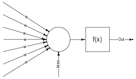
Figure 4: A neuron
An ANN-s is a network of neurons. The network has an input and an output, and it can be trained to provide the right output for a certain input. A neuron is responsible for simple operations, but the whole network can make parallel calculations as the result of its vast parallel structure. The neurons have some inputs with input weights. The inputs are summed up and feeded into a so called transfer function. The output of the transfer function is considered as the output of the neuron. This output can be further connected into the inputs of other neurons resulting in a vast network of neurons. [4] The structure of a neuron is shown on Fig.4.
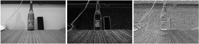
Figure 5: The intensity (left), difference (middle) and orientation (right) values of the pixels of an image
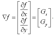
In the presented system three pixel properties will be used in the comparison [5]. These quantities are intensity, gradient magnitude and orientation (I,D,O) Fig.5. Denote the intensity of an arbitrary pixel in location (x;y) as I = f (x;y), the gradient of f (x;y) is defined as
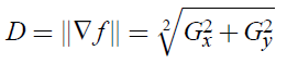
Its magnitude is defined as the variation of f(x,y) and is written as
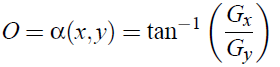
The orientation a(x;y) of the vector f is defined in location (x,y) as
3 The Proposed System for Stereo Matching
3.1 Pixel Pair Matching
The goal of the proposed system is to adjust two cameras so that both of them has the same 3D point projected on the center of their image planes, like the human eyes look at the same spot when trying to assess the distance of a certain object. The following assumptions were made in the choice of the pixels to be compared with each other.
We supposed to have a master(left) and a slave(right) camera (eye). The images provided by these cameras will be referred to as master and slave images. The system adjusts the optical center of the right camera so that the same point P is projected on both of the optical centers, while the master camera is not moving at all. A window of 9x9 pixels is considered as a pixel surrounding. Thus on the master image there is a single pixel with one window. The final task is to find a window on the slave image that matches the window of the master image.
Not all the pixels on the slave image are taken into consideration. In stereo vision if the external and internal parameters of the cameras (such as their position, orientation, and focal length) are known, than for each point on one of the images a line can be given on the other image which will contain the pair of the point seen on the first image. This line is referred to as the epipolar line, providing a constraint to the pixels to be taken into consideration in the matching process [5][6]. We also suppose that there is no vertical rotation or translation between the master and the slave cameras, furthermore the window on the master image is always in the optical center. This yields that the epipolar line on the slave image is always horizontal and passes through the optical center of the slave camera. As a result all the windows of 9x9 pixels on the epipolar line of the slave image will be compared to the single window in the center of the master image, thus the interesting image parts are the 9x9 square on the master image and an Xmax9 band on the slave image, where Xmax is the width of the slave image in pixels.
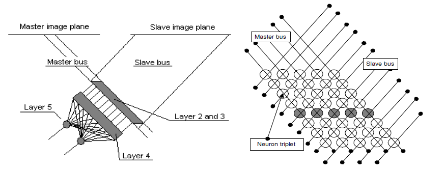
Figure 6: The overview of the proposed ANN (left) and a section of the 3D array holding the neurons of the second layer (right). Each line represents the difference of one window pair.
Color image can be decomposed to three images according to their RGB components. In our system gray scale images are used with intensities varying from 0 to 255. Because the intensity value of each pixel is sensitive to changes in contrast and illumination, comparing only the intensities of the pixels and their surroundings to acquire a matching degree does not give an acceptable result. The gradient of each pixel is also taken into consideration while comparing them. We suppose that three quantities, intensity, difference, orientation (I,D,O) of each pixel are known. The matching degree of a pixel pair pL(xL,yL) and pR(xR,yR) is defined as the average of the absolute difference between the corresponding feature values of the pixels. Denote d(pL, pR) as the matching degree, it can be written in the following form:
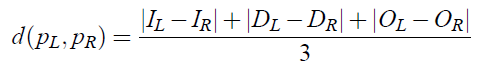
This choice has been made because it gives a true degree of similarity between pixels, it can be computed by an ANN using input weights that are easy to adjust in advance. In the next section the proposed neural structure will be presented along with the description of the chosen input weights and transfer functions.
3.2 Neural Based Structure for Matching and Camera Control
The proposed neural structure is shown on Fig.6 (left). The system is composed of 5 layers. Each layer is responsible for a different task (input, matching degree, decision, output), which yields a clear structure that is easy to understand and further develop. In the first layer we suppose to have the input data from the interesting image regions, i.e. the 9 ¤ 9 square on the master image and the Xmax ¤ 9 band from the slave image. These data are feeded into the input layer of the ANN.
The outputs of the input neurons form two buses, a master and a slave bus, as an analogy of the optic nerves behind the human eyes. The master bus M carries the I, D and O values of the 9x9 window on the master image, thus groups 3 * 9 * 9 = 243 outputs of the input layer. Mi; j denotes the I, D and O values that belong to the pixel pM(i, j) in the master window. The slave bus S carries the I, D and O values of the Xmax * 9 band on the slave image, thus groups 3 * 9 * Xmax outputs of the input layer. Sk; j denotes the I, D and O values that belong to the pixel pS(k; j) in the band on the slave image. The two buses are then crossed in a 3-dimensional array A of 9 * 9 * (Xmax, 8) neuron triplets, which is the second layer of the proposed ANN. A two dimensional section where j is set to a constant value is shown in Fig.6 (right).
In array A each neuron triplet calculates the absolute difference of the I, D and O values with respect to the pixels from which their inputs are arriving from.
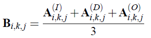
The third layer neurons of the network are situated in a similar 3D array as those in the second layer. The difference is that in the third layer there is only one neuron in each cell of the array. The outputs of the three corresponding neurons in layer 2 are connected to the inputs of the neurons in layer 3. Denote the array containing the third-layer neurons B, then the operation performed by a third layer neuron is described as
This means that the third layer neuron simply calculates the mean value of the outputs coming from the three second-layer neurons. The output is then the same as it was written in Equation 5. In other words, Bi,k,j equals the mean difference between the pixels pM(i, j) and pS(k+i, j). It is to note that if k is increased by one, then B will contain the mean difference between the same pixel on the master image and the next pixel to the right on the slave image.
To compute the matching degree between two pixels, their surroundings also have to be taken into consideration. The array Bi,c,j where c is a constant, contains the average difference between the 81 pixels in the 9 * 9 master window and the cth slave window. To get the matching degree of a pixel pair, simply the mean value of the 81 difference values is calculated, and subtracted from 255, the maximum value of the difference. This is done by the fourth layer of the network, which contains Xmax - 8 neurons with 81 inputs for each of them. The output of the kth neuron equals to the matching degree of the master window and the kth window on the slave image.
Our original goal was to adjust the optical center of the slave camera on the point P projected on the optical center of the master camera. We can say that the goal is achieved when the highest matching degree is given by the Xmax - 8=2th neuron. In other words the highest matching has to occur in the middle neuron of the fourth layer.
It is the task of the fifth layer to decide if the highest matching value is in the middle of the fourth layer, and if not, then in which way it is situated. In the fifth layer there are only two neurons. Both have Xmax - 8 inputs, all the outputs of the fourth layer. One of the neurons tells how far the neuron providing the maximum of the matching degrees is situated to the right, and the other tells the same to the left. Finally a simple control system has to decide if the left one is higher than the right, or inverse, and tell the motor to drive the camera to the appropriate direction.
3.3 Input Weights and Transfer Functions
In order to the structure described above becomes functional, the input weights and transfer functions have to be adjusted. As we have cited in the introduction, no training of the network has been done. Since the neurons perform simple operations, their input weights and transfer functions can be easily pre-adjusted. In this section we are going to present the weights and transfer functions applied in the neural network.
- In the first layer neurons put their inputs to their outputs. They used an input weight of 1, and a linear transfer function.
- In the second layer, each neuron has two inputs. The output is the absolute value of their differences: Output =|Input1|-|Input2|. Thus the input weights are as follows: w1 = 1, w2 = -1 and the transfer function is f (x) = abs(x).
- In the third layer the mean value of three neuron outputs from the second layer is calculated. To perform this operation, the input weights are as follows: w1 = 1=3, w2 = 1=3, w3 = 1=3 and the transfer function is f (x) = x.
- In the fourth layer another mean value is calculated. In this case there are two possibilities. A negative mean value can be calculated where all the 81 input weights are the same, or the inputs can be weighed according to a negative gaussian function, supposing that the pixels close to the center of the window are more important. Negative values are used because the mean difference is smaller at a higher matching degree. In order to have an increasing matching degree with the decreasing difference, matchingdegree=255 - difference is used. In our case each weight has been the same: wi = -1/81; i = [1..81]. A bias of 255-th is used, where th is the threshold of sensitivity. The transfer function is f (x) = sgn(x). The sgn function has been used to eliminate the noise from the matching degrees provided by the fourth layer. The elimination is necessary for the fifth layer to work properly.
- The last, fifth layer is responsible for the decision about the direction of the fourthlayer neuron providing the maximal matching degree. Two neurons are used, one of them having input weights decreasing from the left to the right, and the other one decreasing from the right to the left. The weights become zero just after the input belonging to the central fourth-layer neuron, as shown on Fig.7. The transfer function of this layer is a simple linear function f (x) = x.
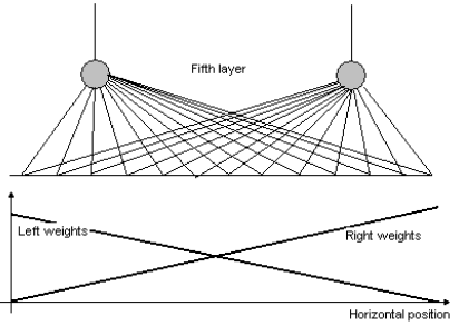
Figure 7: The input weights of the 5th layer are pre-adjusted to increase and decrease with the horizontal position in the left and right neuron respectively.
4 Testing and Evaluation
To evaluate the proposed system, we have made several tests, where the camera system to control was replaced by stereo image pairs taken by digital cameras. The output of the tests was a decision about the direction in which the slave camera had to be rotated. The system also provided a graph of the matching degree according to the horizontal position of the matched window on the slave image.
Here we present two image pairs with the matching degree graphs and the direction suggested by the system.
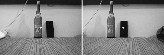
Figure 8: Master image (left) and slave image (right). The image centers are indicated by the white dots on both images. The matching pixel on the slave image is located to the left from the center of the slave image.
On the first image pair the center of the left image corresponds to a pixel that is situated to the left from the center of the right image. This can also be seen on the graph of the matching degree (Figure 9). A threshold is applied to the graph matching degree, and it is feeded into the fifth layer of the ANN. On its output it gives 47530 and 47506 as a degree of directing the slave (right) camera to the left and right respectively. The left value being higher, the camera will turn to the right, which is the desirable motion in this case.
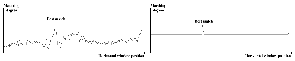
Figure 9: The matching degree of the first image pair before (left) and after(right) applying the threshold. The peak representing the best match is to the left from the center.
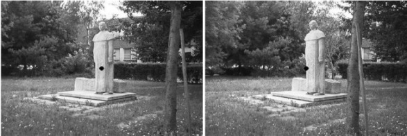
Figure 10: Master image (left) and slave image (right). The image centers are indicated by the black dots on both images. The matching pixel on the slave image is located to the right from the center of the slave image.
On the second pair (Figure 10) of images the center of the left image corresponds to a pixel that is situated to the right from the center of the right image. The matching degrees are shown on Figure 11. Finally the output of the network is 47506 and 47514 for the left and right directions respectively. In this case the value representing the right side is higher, meaning that the slave camera has to be rotated to the right.
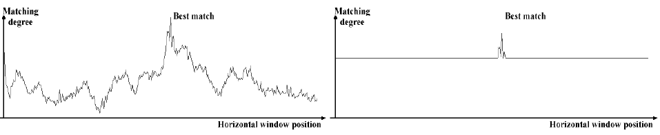
Figure 11: The matching degree of the second image pair before (left) and after(right) applying the threshold. The peak representing the best match is to the right from the center.
5 Conclusion
The presented biologically inspired artificial neural network gives a similar quality of solution to the disparity matching and camera control as other systems. Hence, its vast parallel structure embedded in a neural chip performs the task much faster than conventional PC based simulations.
The system is robust when using pictures coming from a well-calibrated stereo camera pair. It is not sensitive to a change of intensity or focus on one of the images.
The structure of the proposed system is composed of 5 well-distinguished layers resulting in a clear structure that is easy to understand and further develop. The parameters of the neurons are simple to pre-adjust, the computational power of the system comes from its structural build-up, rather than the complexity of the input weights.
Concerning the further developments, the fifth layer of the ANN is intended to be enhanced so that no threshold has to be used in the transfer function of the fourth layer. Furthermore, the density of the input pixels should be decreased on the peripheral regions of the image planes of the cameras. This would decrease the number of neurons used to build up the structure.
References
- T. Kanade, and M. Okutomi A stereo matching algorithm with an adaptive window: theory and experiment. IEEE Trans. Pattern Anal. Machine Intell., 16, 920-932, 1994
- U. R. Dhond, and J. K. Aggarwal Structure from stereo-a review. IEEE Trans. Syst., Man, Cybern., 3, 1489-1510., 1989
- Jung-Hua Wang and Chih-Ping Hsiao On Disparity Matching in Stereo Vision via a Neural Network Framework Proc. Natl. Sci. Counc. ROC(A) Vol. 23, No. 5, 1999. pp. 665-678, 1999
- S. S. Haykin Neural Networks: A Comprehensive Foundation. Prentice Hall, 1998
- D. A. Forsyth, and J. Ponce Computer Vision: A Modern Approach. Prentice Hall, 2002
- I. P. Howard, B. J. Rogers, and A. P. Howard, Binocular Vision and Stereopsis. Oxford University Press, 1995
- H. H. Hagel, and G. A. Orban, Artificial and Biological Vision Systems. Springer Verlag, 1992
- Z. Petres, P. Baranyi, B. Papp and K. Beres, Modeling of Basic Mental Action–Reaction Behavior by Neural Structures. In Proceedings of International Conference on Fuzzy Information Processing, Beijing, China, pages 2:491–496, 2003