
Alexey Shevchenko
Faculty of Computer Science and Technology (CST)
Department of Software Intelligent Systems
Speciality Software systems
Research on methods of game artificial intelligence optimizations, based on more efficient pathfinding by agents
Scientific adviser: Ph.D. Assoc. Alexander Zhuk
Abstract
Content
- Introduction
- 1. Theme urgency
- 2. Local collision avoidance methods
- 2.1 Velocity obstacle
- 2.2 Reciprocal velocity obstacle
- 3. Construction path methods on the navigation mesh
- 3.1 Polygon movement
- 3.2 Polygon edge movement
- 3.3 Polygon vertex movement
- 3.4 Hybrid movement
- 3.5 Path smoothing
- 4. Solving problems using the velocity obstacles methods on the navigation mesh
- 4.1 Providing navigation along the path and simultaneous analysis of possible collisions
- 4.2 Accounting restrictions on passability of the map in collision avoidance
- 4.3 Re-paving the path after collision avoidance
- Conclusion
- References
Introduction
Theory of finding shortest paths has great importance in the modern world. Due to its widespread use, it has recently been intensively developed: along with the improvement of existing methods developed fundamentally new.
There are many optimization problems connected with the search of the shortest paths. As a result - finding a shortest path in the world today is used almost everywhere: from global positioning systems to find the shortest route of city streets and routes between cities, military and civilian systems, autopilot, in travelling services - and up to computer games.
Pathfinding algorithms are divided into two main types.
- Pathfinding on discrete working area (DWA).
- Pathfinding on a graph.
Both classes of algorithms have their advantages and disadvantages, as well as its scope. The first class of algorithms are simple enough, but does not always give good results, so in this paper will be considered second class.
But finding the shortest path is not the only problem. After finding it, some agent must pass this path and not to collide with other agents moving around. To solve this problem, there are also a series of algorithms that allow agents to move with a safe trajectory to their destination with minimal deviations from ideal path and in minimum time.
1. Theme urgency
Modern video games are very complex programs, which are subject to very strict requirements. Everything that happens on the screen should be as realistic and as quickly as possible. If there is no at least one of these requirements, users will be just boring to play that game.
Today there are many different algorithms and techniques of pathfinding and collision avoidance to move on a virtual map. But all of these methods work alone, but are not designed to work together, or do not take into account some minor features. For example, collision avoidance methods do not consider static obstacles, and pathfinding methods do not account the size of agent.
Given all of the above, it is urgent that a combination of pathfinding and collision avoidance mehods on the map provided by the navigation mesh to create the most realistic behavior, logical and fast moving agents on the map.
2. Local collision avoidance methods
2.1 Velocity obstacle
The velocity obstacle [1] of a virtual agent induced by a moving obstacle in a game level is the set of all velocities for the virtual agent that will result in a collision between the virtual agent and the moving obstacle within some short time interval into the future, assuming that the dynamic obstacle maintains a constant velocity. It follows that if the virtual agent chooses a velocity within the region corresponding to the velocity obstacle, then the virtual agent and the moving obstacle will potentially collide. If the velocity chosen is outside the velocity obstacle, then a collision will not occur. A geometric interpretation of a velocity obstacle VOab for a virtual agent A with respect to a virtual agent B corresponding to a cone is shown in Figure 1.

Figure 1 - Velocity obstacle
Unfortunately, the velocity obstacle approach does not work very well for local collision avoidance within a group of virtual agents where each virtual agent is actively changing its velocity to avoid the other virtual agents, since it assumes that other virtual agents may not change their velocities. If all virtual agents were to use velocity obstacles to choose a new velocity, there would be oscillations in the motion of the virtual agents between successive time steps.
2.2 Reciprocal velocity obstacle
The reciprocal velocity obstacle [2] addresses the problem of oscillations caused by the velocity obstacle by allowing for the reactive nature of the other virtual agents. Instead of one virtual agent having to take all the responsibility for avoiding collisions, reciprocal velocity obstacles let a virtual agent take just half of the responsibility for avoiding a collision and assume that the other virtual agent reciprocates by taking care of the other half. The geometric interpretation of a reciprocal velocity obstacle RVOA|B for a virtual agent A with respect to a virtual agent B as a velocity obstacle with its apex translated is shown in Figure 2.

Figure 2 - Reciprocal velocity obstacle
But this method is not perfect. It has some problems, the most significant of which is the problem of reciprocal dances
It shows itself when the agents strongly deviate from their trajectory of movement, so they may be blocked by other agents. To this problem address the optimal reciprocal velocity obstacles [3] and hybrid reciprocal velocity obstacles [4].
3. Construction path methods on the navigation mesh
Navigation mesh - all traversed space consisting of disjoint polygons[5]. The walkable areas can have additional information attached to them. We can then treat this much like we treat a grid. As with a grid, we have a choice of using polygon centers, edges, or vertices as navigation points.
3.1 Polygon movement
As with grids, the center of each polygon provides a reasonable set of nodes for the pathfinding graph. In addition, we have to add the start and end nodes, along with an edge to the center of the polygon we’re in. An example is shown in Figure 3.

Figure 3 - Polygon movement path
In this example, the yellow path is the what we’d find using a pathfinder through the polygon centers, and the pink path is the ideal path.
3.2 Polygon edge movement
Moving to the center of the polygon is usually unnecessary. Instead, we can move through the edges between adjacent polygons. In this example, I picked the center of each edge. The yellow path is what we’d find with a pathfinder through the edge centers, and it compares pretty well to the ideal pink path. An example is shown in Figure 4.

Figure 4 - Polygon edge movement path
3.3 Polygon vertex movement
The shortest way around an obstacle is to go around the corner. This is why we used corners for the visibility graph representation. We can use vertices with navigation meshes. An example is shown in Figure 5.

Figure 5 - Polygon vertex movement path
There’s only one obstacle in the way in this example. When we need to go around the obstacle, the yellow path goes through a vertex, just as the pink (ideal) path does. However, whereas the visibility graph approach would have a straight line from the start point to the corner of the obstacle, the navigation mesh adds some more steps. These steps typically should not go through vertices, so the path looks unnatural, with wall hugging
behavior. An example is shown in Figure .
3.4 Hybrid movement
There aren’t any restrictions on what parts of each polygon can be made into navigation points for pathfinding. You can add multiple points along an edge, and the vertices are good points too. Polygon centers are rarely useful. An example is shown in Figure 6.

Figure 6 - Hybrid movement path
3.5 Path smoothing
Path smoothing is fairly easy with the resulting paths, as long as the movement costs are constant. The algorithm is simple: if there’s line of sight from the navigation point i to point i+2, remove point i+1. Repeat this until there is no line of sight between adjacent points in the path.
What will be left is only the navigation points that go around the corners of obstacles. These are vertices of the navigation mesh. If you use path smoothing, there’s no need to use edge or polygon centers as navigation points; use only the vertices.
In the above examples, path smoothing would turn the yellow path into the pink one. However, the pathfinder has no knowledge of these shorter paths, so its decisions won’t be optimal. Shortening the path found in an approximate map representation (navigation meshes) will not always produce paths that are as good as those found in a more exact representation (visibility graphs).
4. Solving problems using the velocity obstacles methods on the navigation mesh
4.1 Providing navigation along the path and simultaneous analysis of possible collisions
Let the shortest path length N is a sequence of points:
 , (1)
, (1)
where  – the starting waypoint,
 – intermediate waypoints,
 – endpoint.
When moving along the route agent at each time point should move at a speed:
 , (2)
, (2)
where i – index of the last passed waypoint,
 – the velocity of agent,
 – valuation of vector.
The reciprocal velocity obstacles method ignores data of the destination point. The input data are:
- desired speed vector of each agent (
 );
); - current velocity vector of each agent (
 ).
).
The result of applying this method is the current velocity vector for each agent. Obviously, for the continuation of the movement on the planned route, the desired velocity vector  need to be recalculated at each time:
 , (3)
, (3)
where  – current position of agent on the map.
The described situation with velocity vectors is shown in Figure 7.

Figure 7 – Calculation of agent's velocity vector when used pathfinding methods and reciprocal velocity obstacle methods for map navigation
4.2 Accounting restrictions on passability of the map in collision avoidance
Route M is laid so that the moving agent on it may touch obstacles, but its trajectory is always within walkable area map.
At the same time, when virtual agent avoiding collision, it may select such velocity that after a maneuver it releases the bounds of terrain.
Reciprocal velocity obstacles method allows to calculate the velocity vector of virtual agent, which guarantees the absence of collisions with obstacles. Thus, if we represent the boundaries of the terrain as an obstacle to reciprocal velocity obstacles method, then this problem will be solved.
Each polygon of navigation mesh can be divided into non-overlapping triangles so that their total area is equal to the area of the terrain. Partition of all navigation mash polygons into triangles will be called triangulation. The example of navigation mesh and it triangulation are shown on Figure 8.
 and it triangulation (b). Shaded polygons correspond to walkable areas")
Figure 8 – Navigation mesh (a) and it triangulation (b). Shaded polygons correspond to walkable areas
Each of K triangles is a complete graph. If all these triangles combined into one graph, we obtain a graph consisting of K connected components. If combine this graph vertices that have the same coordinates, we obtain a connected graph with multiple edges. Let the resulting graph have K vertices and let M - adjacency matrix of the graph. If on the matrix M perform the following operation
 , (4)
, (4)
it will be the same with the removal of the resulting graph of multiple edges. The resulting graph will contain only connected components, each component is a cycle - boundary loop of obstacles on the map.
4.3 Re-paving the path after collision avoidance
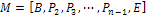
One of the properties of the route, laid on the navigation mesh is that every two adjacent points in it are in sight of each other, so there are no edges, which would cross segment  .
.
As discussed earlier, after collision avoidance velocity vector to the next waypoint would require recalculation. However, it is possible that after avoiding there is an edge, which intersects the segment  . The presence of such a segment will be considered an indicator of the need to re-calculate the route from point to point E.
Conclusion
Master's work is devoted to solving actual scientific problem of combining the pathfinding methods and collision avoidance methods. In the context of work carried out:
- An analysis of existing pathfinding methods and collision avoidance.
- For selected methods and algorithms discussed the possibility of their combining.
- A number of tests and the basic problems of the using methods of local collision avoidance on the navigation mesh.
- Proposed the possibilities of solving found problems. Implementing these solutions will apply the method reciprocal velocity obstacles to local collision avoidance of virtual agents when moving on a map, provided by navigation mesh.
Further studies focused on the following aspects:
- Adding agent priorities in local collision avoidance methods.
- Accounting the size of the agent in planning the route on navigation mesh.
This master's work is not completed yet. Final completion: December 2014. The full text of the work and materials on the topic can be obtained from the author or his head after this date.
References
- P. Fiorini and Z. Shiller,
Motion planning in dynamic environments using velocity obstacles
, Int. Journal of Robotics Research, vol. 17, no. 7, pp. 760-772, 1998. - van den Berg, J., Lin, M., Manocha, D.: Reciprocal Velocity Obstacles for real-time multi-agent navigation. In: IEEE Int. Conf. on Robotics and Automation, pp. 1928–1935 (2008).
- J. Snape , J. van den Berg , S. J. Guy , D. Manocha, The Hybrid Reciprocal Velocity Obstacle, IEEE Transactions on Robotics, v.27 n.4, p. 696-706, August 2011.
- van den Berg, J., Guy, S., Lin, M., Manocha, D. (2011). Reciprocal n-body collision avoidance. In C. Pradalier, R. Siegwart, G. Hirzinger (Eds.), Robotics Research: The 14th International Symposium ISRR (pp. 3-19). Berlin, Germany: Springer.
- Marcelo Kallmann, Shortest paths with arbitrary clearance from navigation meshes, Proceedings of the 2010 ACM SIGGRAPH/Eurographics Symposium on Computer Animation, July 02-04, 2010, Madrid, Spain.