Synonyms
Video Compression Techniques
Definition
Video coding techniques and standards are based on a set of principles that reduce the redundancy in digital video.
Introduction
Digital video has become main stream and is being used in a wide range of applications including DVD, digital TV, HDTV, video telephony, and teleconferencing. These digital video applications are feasible because of the advances in computing and communication technologies as well as efficient video compression algorithms. The rapid deployment and adoption of these technologies was possible primarily because of standardization and the economies of scale brought about by competition and standardization. Most of the video compression standards are based on a set of principles that reduce the redundancy in digital video.
Digital video is essentially a sequence of pictures displayed overtime. Each picture of a digital video sequence is a 2D projection of the 3D world. Digital video thus is captured as a series of digital pictures or sampled in space and time from an analog video signal. A frame of digital video or a picture can be seen as a 2D array of pixels. Each pixel value represents the color and intensity values of a specific spatial location at a specific time. The Red-Green-Blue (RGB) color space is typically used to capture and display digital pictures. Each pixel is thus represented by one R, G, and B components. The 2D array of pixels that constitutes a picture is actually three 2D arrays with one array for each of the RGB components. A resolution of 8 bits per component is usually sufficient for typical consumer applications.
The Need for Compression
Consider a digital video sequence at a standard definition TV picture resolution of 720 * 480 and a frame rate of 30 frames per second (FPS). If a picture is represented using the RGB color space with 8 bits per component or 3 bytes per pixel, size of each frame is 720 * 480 * 3 bytes. The disk space required to store one second of video is 720 * 480 * 3 * 30 = 31.1 MB. A one hour video would thus require 112 GB. To deliver video over wired and/or wireless networks, bandwidth required is 31.1 * 8 = 249 Mbps. In addition to these extremely high storage and bandwidth requirements, using uncompressed video will add significant cost to the hardware and systems that process digital video. Digital video compression is thus necessary even with exponentially increasing bandwidth and storage capacities.
Fortunately, digital video has significant redundancies and eliminating or reducing those redundancies results in compression. Video compression can be lossy or loss less. Loss less video compression reproduces identical video after de-compression. We primarily consider lossy compression that yields perceptually equivalent, but not identical video compared to the uncompressed source. Video compression is typically achieved by exploiting four types of redundancies: (1) perceptual, (2) temporal, (3) spatial, and (4) statistical redundancies.
Perceptual Redundancies
Perceptual redundancies refer to the details of a picture that a human eye cannot perceive. Anything that a human eye cannot perceive can be discarded without affecting the quality of a picture. The human visual system affects how both spatial and temporal details in a video sequence are perceived. A brief overview of the human visual system gives us an understanding of how perceptual redundancies can be exploited.
The Human Visual System
The structure of the human eye is shown in Fig. 1.
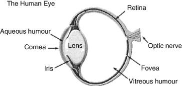
Figure 1 – Structure of the human eye
The human visual system responds when the incoming light is focused on the retina. The photoreceptors in the eye are sensitive to the visible spectrum and generate a stimulation that results in perception. The retina has two types of photo receptors (1) rods and (2) cones. Human eye has about 110 million rods and about seven million cones. The rods and cones respond differently to the incident light. Rods are sensitive to the variations in intensity (lightness and darkness) and cones are sensitive to color. Rods function well under low illumination and cones function under well-lit conditions. There are three types of cones, Red, Green, Blue each sensitive to the different bands of the visible spectrum. About 64% of the cones are red, 32% green, and about 4% blue. The cones, however, are not uniformly distributed on the retina. The fovea, the central area of the retina, has more green cones than reds and blues resulting in different sensitivity to different bands of the visual spectrum. This makes the human eye more sensitive to the mid spectrum; i.e., the incoming blues and reds have to be brighter than greens and yellows to give a perception of equal brightness. Because of the large number of rods, the human eye is more sensitive to variations in intensity than variation in color.
The RGB color space does not closely match the human visual perception. The YCbCr color space (also known as YUV), where Y gives the average brightness of a picture and Cb and Cr give the chrominance components, matches the human visual perception better. The YCbCr representation thus allows exploiting the characteristics of the visual perception better.
Sensitivity to Temporal Frequencies
The eye retains the sensation of a displayed picture for a brief period time after the picture has been removed. This property is called persistence of vision. Human visual persistence is about 1/16 of a second under normal lighting conditions and decreases as brightness increases. Persistence property can be exploited to display video sequence as a set of pictures displayed at a constant rate greater than the persistence of vision. For example, movies are shown at 24 frames per second and require very low brightness levels inside the movie theater. The TV, on the other hand, is much brighter and requires a higher display rate. The sensitivity of the eye to the frame rate also depends on the content itself. High motion content will be more annoying to the viewer at lower frame rates as the eye does not perceive a continuous motion. The persistence property can be exploited to select a frame rate for video display just enough to ensure a perception of continuous motion in a video sequence.
Sensitivity to Spatial Frequencies
Spatial frequencies refer to the changes in levels in a picture. The sensitivity of the eye drops as spatial frequencies increase; i.e., as the spatial frequencies increase, the ability of the eye to discriminate between the changing levels decreases. The eye can resolve color and detail only to a certain extent. Any detail that cannot be resolved is averaged. This property of the eye is called spatial integration. This property of the eye can be exploited to remove or reduce higher frequencies without affecting the perceived quality. The human visual perception thus allows exploitation of spatial, temporal, and perceptual redundancies.
Video Source Format
The input to video compression algorithms typically uses the YCbCr color space as this representation lends itself better to exploiting the redundancies of the human visual system. The RGB primaries captured by an acquisition device such as a camera are converted into the YCbCr format. Figure 2 shows the luma and chroma sampling for the YCbCr formats. The YCbCr 4:4:4 format has four Cb and four Cr pixels for every 2 * 2 block of Y pixels, the YCbCr 4:2:2 format has two Cb and two Cr pixels for every 2 * 2 block of Y pixels, and the YCbCr 4:2:0 format has one Cb and one Cr pixels for every 2 * 2 block of Y pixels. All the three formats have the Y component at the full picture resolution. The difference in the formats is that the YCbCr 4:2:2 and YCbCr 4:2:0 formats have the chroma components at a reduced resolution. The human eye cannot perceive the difference when chroma is sub sampled. In fact, even the YCbCr 4:2:0 format with chroma one fourth of the luma resolution is sufficient to please the human eye. The YCbCr 4:2:0 format is the predominantly used format and is used in applications such as DVD, digital TVs, and HDTVs. The YCbCr 4:2:2 is typically used for studio quality applications and YCbCr 4:4:4 is hardly used. The use of YCbCr 4:2:0 instead of the RGB color space represents a 50% reduction in image size and is a direct result of exploiting the perceptual redundancies of the human visual system.
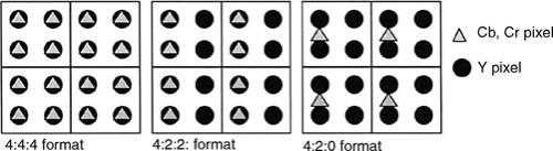
Figure 2 – Video source formats
Exploiting Temporal Redundancies
Since a video is essentially a sequence of pictures sampled at a discrete frame rate, two successive frames in a video sequence look largely similar. Figure 3 shows two successive pictures in a video. The extent of similarity between two successive frames depends on how closely they are sampled (frame interval) and the motion of the objects in the scene. If the frame rate is 30 frames per second, two successive frames of a news anchor video are likely to be very similar. On the other hand, a video of car racing is likely to have substantial differences between the frames. Exploiting the temporal redundancies accounts for majority of the compression gains in video encoding.
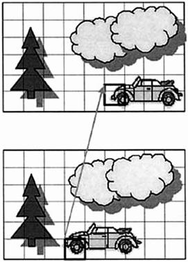
Figure 3 – Successive frames in a video
Since two successive frames are similar, taking the difference between the two frames results in a smaller amount of data to be encoded. In general, the video coding technique that uses the data from a previously coded frame to predict the current frame is called predictive coding technique. The computation of the prediction is the key to efficient video compression. The simplest form of predictive coding is frame difference coding, where, the previous frame is used as a prediction. The difference between the current frame and the predicted frame is then encoded. The frame difference prediction begins to fail as the object motion in a video sequence increases resulting in a loss of correlation between collocated pixels in two successive frames.
Object motion is common in video and even a small motion of 1-2 pixels can lead to loss of correlation between corresponding pixels in successive frames. Motion compensation is used in video compression to reduce the correlation lost due to object motion. The object motion in the real world is complex but for the purpose of video compression, a simple translational motion is assumed.
Block Based Motion Estimation
If we observe two successive frames of a video, the amount of changes within small N * N pixel regions of an image are small. Assuming a translational motion, the N * N regions can be better predicted from a previous frame by displacing the N * N region in the previous image by an amount representing the object motion. The amount of this displacement depends on relative motion between the two frames. For example, if there is a five pixel horizontal motion between the frames, it is likely that a small N * N region will have a better prediction if the prediction comes from an N * N block in the previous image displaced by five pixels. The process of finding a predicted block that minimizes the difference between the original and predicted blocks is called motion estimation and the resulting relative displacement is called a motion vector. When motion compensation is applied to the prediction, the motion vector is also coded along with the pixel differences.
Video frames are typically coded one block at a time to take advantage of the motion compensation applied to small N * N blocks. As the block size decreases, the amount of changes within a block also typically decrease and the likelihood of finding a better prediction improves. Similarly, as the block size increases, the prediction accuracy decreases. The downside to using a smaller block size is that the total number of blocks in an image increases. Since each of the blocks also has to include a motion vector to indicate the relative displacement, the amount of motion vector information increases for smaller block sizes.
The best prediction for a given block can be found if the motion of the block relative to a reference picture can be determined. Since translational motion is assumed, the estimated motion is given in terms of the relative displacement of a block in the X and Y planes. The process of forming a prediction thus requires estimating the relative motion of a given N * N block. A simple approach to estimating the motion is to consider all possible displacements in a reference picture and determine which of these displacements gives the best prediction. The best prediction will be very similar to the original block and is usually determined using a metric such the minimum sum of absolute differences (SAD) of pixels or the minimum sum of squared differences (SSD) of pixels. The SAD has lower computational complexity compared to the SSD computation and equally good in estimating the best prediction. The number of possible displacements (motion vectors) of a given block is a function of the maximum displacement allowed for motion estimation. Figure 4 shows the region of a picture used for motion estimation. If D max is the maximum allowed displacement in the X and Y directions, the number of candidate displacements (motion vectors) are (1 + 2D max)*(1 + 2D max). An N * N block requires N*N computations for each candidate motion vector, resulting in extremely high motion estimation complexity. Complexity increases with the maximum allowed displacement. Depending on the motion activity of the source video, D max can be appropriately selected to reduce the motion estimation complexity without significantly affecting the quality of the prediction. Fast motion estimation has been an active area of research and a number of efficient algorithms have been developed.
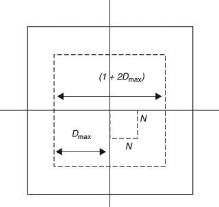
Figure 4 – Motion estimation
Exploiting Spatial Redundancies
In natural images, there exists a significant correlation between neighboring pixels. Small areas within a picture are usually similar. Redundancies exist even after motion compensation. Exploiting these redundancies will reduce the amount of information to be coded. Prediction based on neighboring pixels, called intra prediction, is also used to reduce the spatial redundancies. Transform techniques are used to reduce the spatial redundancies substantially. The spatial redundancy exploiting transforms such as the discrete cosine transform (DCT), transform an N * N picture block into NxN block of coefficients in another domain called the frequency domain. The key properties of these transforms that make them suitable for video compression are: (1) energy compaction and (2) de-correlation. When the transform is applied, the energy of an N * N pixel block is compacted into a few transformed coefficients and the correlation between the transformed coefficients is also reduced substantially. This implies significant amount of information can be recovered by using just a few coefficients. The DCT used widely in image and video coding has very good energy compaction and de-correlation properties. The transform coefficients in the frequency domain can be roughly classified into low, medium, and high spatial frequencies. Figure 5 shows the spatial frequencies of an 8 * 8 DCT block. Since the human visual system is not sensitive to the high spatial frequencies, the transform coefficients corresponding to the high frequencies can be discarded without affecting the perceptual quality of the reconstructed image. As the number of discarded coefficients increases, the compression increases, and the video quality decreases. The coefficient dropping is in fact exploiting the perceptual redundancies. Another way of reducing the perceptual redundancies is by quantizing the transform coefficients. The quantization process reduces the number of levels while still retaining the video quality. As with coefficient dropping, as the quantization step size increases, the compression increases, and the video quality decreases.
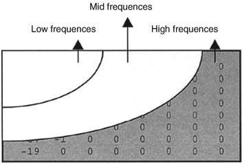
Figure 5 – DCT spatial frequencies
Exploiting Statistical Redundancies
The transform coefficients, motion vectors, and other data have to be encoded using binary codes in the last stage of video compression. The simplest way to code these values is by using fixed length codes; e.g., 16 bit words. However, these values do not have a uniform distribution and using fixed length codes is wasteful. Average code length can be reduced by assigning shorter code words to values with higher probability. Variable length coding is used to exploit these statistical redundancies and increase compression efficiency further.
Hybrid Video Coding
Video compression algorithms use a combination of the techniques presented in order to reduce redundancies and improve compression. The hybrid video compression algorithms are a hybrid of motion compensation and transform coding. Figure 6 shows the key components of a generalized hybrid video encoder. The input source video is encoded block-by-block. The first frame of video is typically encoded without motion compensation as there is no reference frame to use for motion compensation. The transform module (T) converts the spatial domain pixels into transform domain coefficients. The quantization module (Q) applies a quantizer to reduce the number of levels for transformed coefficients. The quantized coefficients are encoded using variable length coding module (VLC). The encoded block is de-quantized (Q in -1) and the inverse transform (T in -1) is applied before saving in a frame store so that the same picture data is used as a reference at the encoder and the decoder. Subsequent pictures can use motion compensation to reduce temporal redundancies. The motion estimation module (ME) uses the source frame and a reference frame from the frame store to find a motion vector that gives a best match for a source picture block. The motion compensation (MC) module uses the motion vector and obtains a predicted block from the reference picture. The difference between the original block and the predicted block, called the prediction error, is then encoded.
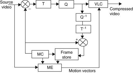
Figure 6 – Hybrid video encoder
Most of the video compression standards used today are based on the principles of hybrid video coding. The algorithms differ in the specifics of the tools used for motion estimation, transform coding, quantzation, and variable length coding. The specifics of the important video compression algorithms used today are discussed in the related short articles.
The MPEG Standardization Process
The MPEG video standards are developed by experts in video compression working under the auspice of the International Organization for Standardization (ISO). The standards activity began in 1989 with the goal of developing a standard for a video compression algorithm suitable for use in CD-ROM based applications. The committee has since standardized MPEG-1, MPEG-2, MPEG-4, and MPEG-4 AVC also known as H.264. Figure 7 shows the timeline for standards development. The key to the success and relevance of the MPEG standards is the standardization process.
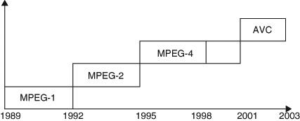
Figure 7 – MPEG video standards timeline
The MPEG process is driven by the industry with participation and contributions from the academia. The MPEG process is open and is essentially a competition among the proponents of a technology. The competing tools and technologies are experimentally evaluated and the best technology is selected for standardization. The standardization process may also combine competing proposals in developing an efficient solution. This process ensures that only the best technologies are standardized and keeps the standards relevant to the industry needs.
Cross-References
MPEG-4 Advanced Video Compression (H.264)
References
1. B. Furht, "dMultimedia Systems: An Overview," IEEE Multimedia, Vol. 1, 1994, pp. 47-59.
2. B. Furht, J. Greenberg, R. Westwater, "Motion Estimation Techniques for Video Compression," Kluwer Academic, Norwell, MA, 1996.
3. D.L. Gall, "MPEG: a Video Compression Standard for Multimedia Applications," Communications of the ACM, Vol. 34, 1991, pp. 46-58.
4. B.G. Haskell, A. Puri, A.N. Netravali, "Digital Video: An Introduction to MPEG-2," Chapman & Hall, London, 1996.
5. M. Liou, "Overview of the P-64 kbit/s Video Coding Standard," Communications of the ACM, Vol. 34, 1991, pp. 59-63.
6. A.N. Netravali and B.G. Haskell, "Digital Pictures - Representation, Compression and Standards," 2nd Edn, Plenum, New York, 1995.
7. D. Marpe, H. Schwartz, and T. Weigand, "Overview of the H.264/ AVC Video Coding Standard," IEEE Transactions on Circuits and Systems for Video Technology, Vol. 13, No. 7, July 2003, pp. 560-575.
8. J.L. Mitchell, W.B. Pennebaker, C.E. Fogg, D.J. LeGall, "MPEG Video Compression Standard," Digital Multimedia Standards Series, Chapman & Hall, London, 1996, pp. 135-169.
9. F. Pereira, T. Ebrahimi, "The MPEG-4 Book," IMSC, Prentice-Hall PTR, 2002.
10. W.B. Pennebaker and J.L. Mitchell, 'JPEG Still Image Data Compression Standard," Kluwer Academic, Dordecht, 1992.
11. K.R. Rao and P. Yip, "Discrete Cosine Transform: Algorithms, Advantages, Applications," Academic, London, 1990, ISBN0-12-580203-X.
12. I. Richardson, "H.264 and MPEG-4 Video Compression," Wiley, London, 2003.