
Content
- Introduction
- 1. Actuality
- 2. Objective
- 3. System structure analysis
- 3.1 Rationale for sensor choice, and sensor operating principle
- 3.2 Rationale for structural scheme choice
- 4. Programal methods for amplitude determining
- 4.1 Discrete Fourier Transform
- 4.2 Root mean square
- 4.3 Trigonometric approximation
- 4.4 Choice of amplitude determining method
- Conclusion
- List of sources
Introduction
Recently, in bread-making factories, an bulk method of storing flour has become increasingly popular. The reason for increasing the popularity of the bulk method is that the bulk storage and transportation of flour in comparison with the traditional method of storage and transportation has several advantages:
- exclusion of heavy physical work, the entire process is mechanized;
- automation of the process is possible;
- saving on tare;
- reduces the spray (loss) of flour;
- flour is aerated, its quality improves;
- the sanitary condition of the production of bakery products improves;
- operating costs are reduced;
- for large and medium-sized bakery enterprises, electricity is saved;
- saving area.
1. Actuality
The profit of the enterprise to a large extent depends on the price and quantity of flour purchased and how rationally it is consumed. In addition, a subjective estimate of the amount of flour gives a large error in determining the residues (up to two to three tons per silage). The fact is that different types of flour have different density, and if rye flour can be loaded into silage up to 30-31 tons, then flour of the highest grade - up to 35 tons. In addition, in the process of pumping flour in the lower cone-shaped part of the silo, voids are formed, sometimes large in volume, which are not visible from above through the thickness of the flour, even with a lantern. That is why the automation of the task of the shift and daily accounting of the arrival-consumption of flour becomes important. In the bakery project that was put into operation in the early 1970s, such automation was envisaged on the basis of the technical means available at that time. In some factories, automation was introduced, but it did not work well or did not work at all, at other plants it was not implemented, although it was envisaged in the project.
2. Objective
The main goal of the work is to develop a system that allows real-time monitoring of the amount of flour in each silo, using modern hardware and software.
3. System structure analysis
The basic idea of building a system is to record the current value of the weight of the silos according to a specified schedule, or at the request of the operator, and save it in the database.
3.1 Rationale for sensor choice, and sensor operating principle
A magnetoanisotropic sensor was chosen as the primary measuring transducer. Advantages of magnetoanisotropic force transducer are high sensitivity and natural oscillation frequency, power and level of the output signal, high accuracy of measurement, reliability of design, simplicity and low cost of manufacture, low sensitivity to ambient temperature.[1]
The principle of operation of magnetoanisotropic sensors is as follows. Under the influence of external mechanical stresses, the magnetic properties of the material undergo changes in all directions with different intensities and different signs, depending on the magnitude of the external magnetic field, i.e. the magnetic anisotropy of the material changes.
The sensors are arranged as follows. Two mutually perpendicular windings are located in the closed magnetic circuit (Fig. 1). For this purpose, in the magnetic circuit for the windings, four holes are made, located symmetrically at the corners of the square or rectangle. Each of the windings is stacked in two diagonally opposite holes. The measured load is applied at an angle of 45° to the plane of each winding.
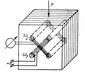
Figure 1 – Magnetoanisotropic sensor
The magnetizing winding ω1 is supplied with alternating current, to the second winding ω2 (measuring), a measuring device or other sensitive organ is connected.
When an alternating current flows through the magnetizing winding, a magnetic flux is created, the distribution pattern of which is shown in Fig.2.[2]
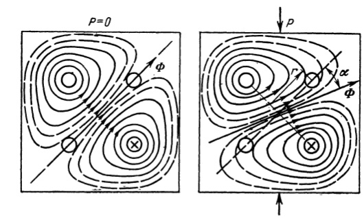
Figure 2 – Distribution pattern of magnetic flux
If the sensor magnetic path is made of magnetically isotropic material and the holes are symmetrically located, then in the absence of loading, the magnetic flux lines, closing, do not cross the measuring winding and, therefore, do not induce an emf in it.
3.2 Rationale for structural scheme choice
The block diagram of the device being developed is presented in Fig. 3
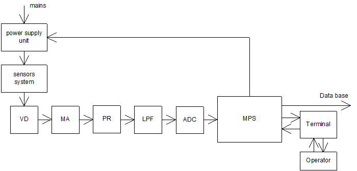
Figure 3 – Block diagram
In this block diagram, the power supply is a sinusoidal signal generator, with a generation frequency of 400 Hz fed from the network.
The sensor system block consists of all sensors used in the system, their excitation windings are connected in parallel, and the measuring windings are connected in series by four, respectively, to the sensors used for weighing one silo, and in parallel to the others. The output of each group of four sensors is connected to the voltage divider, since the sum of the sensor outputs can reach very high values.
From the voltage divider, the signal is applied to a measuring amplifier, which is a two-stage differential amplifier on three operational amplifiers. It provides effective suppression of in-phase noise, as well as has a very high input voltage, and low output. The signal is then rectified by a precision rectifier, which is a full-wave rectifier with a single rectifying unit. The rectified signal is fed to the active low-pass filter of the second order, which performs three functions simultaneously:
- reduction of high-frequency interference;
- smoothing of the rectified signal;
- creating the range of the output signal to the measurement range of the ADC;
From a low-pass filter, the signal is transferred to a microcontroller with a built-in ADC, in which the voltage value is converted to the weight value of the silo and output to the terminal and to the enterprise database.
The problem of determining the signal amplitude can also be solved in a different way. The block diagram of the alternative method is shown in Fig. 4:
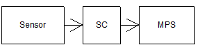
Figure 4 – Alternative construction of a measuring channel
Where SC is scaling converter.
In this scheme it is assumed that the sensor signal is converted into a digitally convenient form by means of a scaling converter and fed to the analog input of the microcontroller. With such a scheme, a harmonic signal acts on the input of the microcontroller, and therefore the use of the instantaneous value does not make sense. However, if a series of measurements are made and an array of time samples is formed from the measurement results, it is possible to programmatically determine the amplitude of the measured signal. Figure 5 shows an example of implementation of this method:
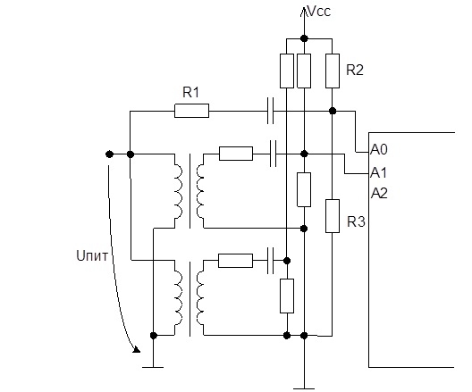
Figure 5 – Circuit implementation
As sensors here are magnetoanisotropic pressure sensors, which are designated as transformers. Since these sensors give a high signal amplitude, a resistive divider can be used as the scaling converter. However, if we simply reduce the amplitude of the signal, then the input of the microcontroller will receive only a half-wave of the sinusoid. In order for the microcontroller to correctly receive the signal, it is necessary to create an offset. Thus, resistors R2 and R3 specify a constant offset equal to half of the maximum level perceived by the MC, and R1 and R3 are voltage dividers that reduce the amplitude of the signal. Thus, a signal acts on the input of the microcontroller, the oscillogram of which is shown in Fig. 6:
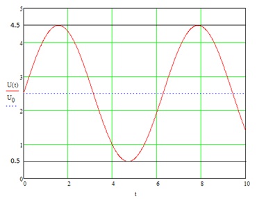
Figure 6 – Input oscillogram
In Fig. 6. It is seen that the constant offset of the signal is 2.5V, and the maximum admissible amplitude of the input signal is 2V.
Thus, when implementing an alternative method of constructing a measuring channel, it becomes possible to achieve a number of advantages:
- serious hardware simplification;
- increase in the reliability of the scheme, due to the reduction in the number of components included in its composition;
- elimination of errors introduced by the measuring channel;
- complete elimination of high-frequency and low-frequency errors;
- increase the speed of the system, due to the fact that in the low-pass filter, to obtain a constant signal level, you need a large capacitor, because of which the measurement time can be up to 0.2 s;
- measurement takes place not only in the amplitude of the measuring winding of the sensor, but also in the supply winding, which also allows monitoring the changes in the sensor supply voltage, and correcting the processing of the results. This significantly reduces the requirements for the accuracy of providing the amplitude of the supply signal generator.
4. Programal methods for amplitude determining
In the case where it is required to programmatically determine the amplitude of a harmonic signal from an array of time samples, an important task is to select the method that is best suited for this, based on the conditions under which the array of samples was generated. For example, the method of direct determination of the amplitude of a harmonic, by determining the maximum and minimum values in an array, will have a high error if there is a disturbance in the signal, or if there is insufficient number of points for one period of the harmonic.
Consider several methods for determining the amplitude of a harmonic signal, as well as their advantages and disadvantages.
4.1 Discrete Fourier Transform
In general, the Discrete Fourier Transform (DFT) is used for spectral analysis of signals, and has the form[3]:
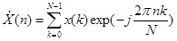 (1)
(1)However, in this case, we are not interested in the spectrum of the signal, but in only one spectral count, and therefore, it is unhelpful to calculate the DFT for the whole spectrum, especially since it can take quite a long time. For this reason, instead of the full one, it is better to use the DFT for one spectral reference.
To implement this approach, it should select the signal sampling period so that in one signal period there are an integer number of time samples. In this case, the number of the desired harmonic will be just the number of time samples per signal period.
Herewith, it is important to understand that the resulting signal amplitude as a result of the DFT will be proportionally different from the actual signal amplitude. For the determination of this proportion, it is also necessary to produce a DFT for the zero harmonic. The obtained value of the zero harmonic is used as the reference value, since It is known that it corresponds to twice the value of the constant component. Then the formula for determining the amplitude of the desired harmonic:
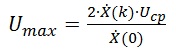 (2)
(2)Where k is the number of the desired harmonic.
The advantages of this method are that you can accurately determine the amplitude of the signal, while completely ignoring the entire spectrum of the signal, except for a single frequency, which is convenient in situations where there are pickups or high-frequency noises.
However, in order to fulfill the condition of an integer number of time samples for the period of the signal, it is necessary to know very accurately the frequency of the given harmonic (with an accuracy not worse than 0.01%), otherwise, due to the very high slope of the characteristic, there will be a large error. Therefore, this method is suitable only in cases where it is possible to determine the signal frequency in advance with high accuracy, or when the signal is generated by a source with very high frequency stability.
4.2 Root mean square
In this method, the amplitude value of the harmonic is determined by the formula:[4]:
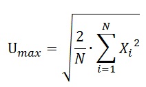 (3)
(3)An important feature of the method is that, for maximum accuracy, it is recommended to use an integer number of signal periods, but with software tools it is easy to determine in the array the points that are most convenient to take as the start and end points.
In addition, an important feature is that for the implementation of this method, it is not necessary to set the signal to a constant offset, so that the entire range of the harmonic is within the measurement range of the ADC. On the contrary, it is possible to pass a signal through a separating capacitor, or the high-pass filter before digitization. For the half-wave signal obtained, the amplitude is:
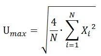 (4)
(4)This approach may be useful if an ADC with a small bit capacity is used, since the entire range of the ADC can work for one half-wave harmonic, instead of the full swing.
4.3 Trigonometric approximation
This method is based on the idea of interpolation by the Fourier polynomial, which has the form[5]:
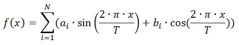 (5)
(5)However, the use of such a polynomial differs little from the usual Fourier analysis, and when it is taken into account that the assumed signal is harmonic, in order to obtain the signal amplitude, it is sufficient to programmatically exclude the constant component from the signal and calculate the coefficient a using the formula:
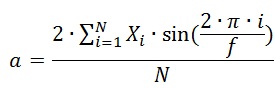 (6)
(6)As in the case of the DFT, to realize this method it is necessary to know the signal frequency in advance, but the accuracy requirements here are much lower (the accuracy of determining the frequency should be no worse than 0.1%). In addition, it is important to ensure that the phase of the approximating sinusoid coincides with the phase of the investigated harmonic. Also, for maximum accuracy, you should select from a source data set such a fragment for analysis, in which the first point is the beginning of the period, and the last is the end of the period.
One of the important advantages of the method is the compensation of the quantization error, so when modeling this algorithm, it was found that a harmonic signal, digitized by 32 quantization levels, can be reconstructed to within a tenth of a percent if there are more than hundreds of points per signal period.
4.4 Choice of amplitude determining method
Since the sensor has a large value of the output voltage, the signal-to-noise ratio is high enough and therefore there is no need to use sophisticated algorithms to ignore noise. Therefore, the method of determining the root-mean-square value looks more rational.
Conclusion
In this abstract, a method for calculating the consumption of flour was described. A sensor is selected, with which the silo mass will be determined and two variant for constructing the measuring channel are suggested. Also, for a variant of a measuring channel based on software determination of the output signal of a sensor, three methods for calculating the amplitude of the signal are reviewed, and one that is more rational is chosen based on the conditions of the task.
This master's work is not completed yet. Final completion: June 2018. The full text of the work and materials on the topic can be obtained from the author or his head after this date.
List of sources
- Дубинин А.Е. Магнито-анизотропные преобразователи силы. – М.: Энерноатомиздат, 1991. – 112с.
- Шевченко Г.И. Магнито-анизотропные датчики. – М.: Энергия, 1967. -73с.
- Александров В.А. Преобразование Фурье: Учеб. пособие. Новосибирск: НГУ, 2002.- 62 с.
- Р.Фано Передача информации. Статическая теория связи. Пер. с англ. И.А.Овсеевича и М.С. Пинскера, под науч. ред. Р.Л.Добрушина. М.: Мир, 1965. – 440с.
- Вержбицкий В.М. Численные методы. – М.: Высшая школа, 2001. – 382с.
- Бауманн Э. Измерение сил электрическими методами. – М.: Мир, 1978. – 423с.