3.1 Introduction
Once image data have been brought into the computer, they are nothing more than numbers that can be manipulated with all the arithmetic and logic capabilities of the computer. When we use images as variables, we call the operations performed algebraic. An algebraic operation can be of one of two types, pointwise or matrix. Both operations can be described by the following annotation:
X opn Y = Z
X and Y can be images or scalars (numbers), and Z must be an image. A pointwise operation, opn, is performed between each corresponding element of X and Y. The matrix type of operation is more complex and involves a detailed series of steps that will be discussed later. We make an assumption that both X and Y, if images, have the same dimension, or spatial resolution. The equation above, as a linear process, is illustrated graphically in Figure 3.1.
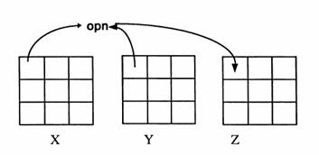
Figure 3.1 Linear algebraic operation between images.
Recall that an image is represented as an array of numbers that is spatially arranged in the same way. As an example of a linear algebraic operation, let's say that we have two images of the same scene. In one of the images, we see a room, possibly in a warehouse. In the other image we see the warehouse with a person in the picture. If we let one image be stored in the global image variable X and the other in Y, and we let opn be subtraction, then the Z image result of the algebraic operation will be a picture of all O's (black) with values only at the pixel locations that were different between the X and Y images. We may also assume that the row and column limit variables (Number_of_Rows, Number_of_Columns) are available as globals as well.
Figure 3.2 illustrates the results of an image subtraction where the second image is subtracted from the first.
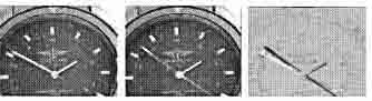
Figure 3.2 Image subtraction example.
As a further example of pixel algebra, consider the brightness control of your monitor. This control scales the overall brightness of the display in proportion to its setting. In the same way, we can multiply each pixel in an image by a constant and thus increase or decrease the value and, correspondingly, the overall brightness of the image.
3.2 Arithmetic Operations
The arithmetic operations between images include addition, subtraction, multiplication, and division. In all cases, we replace opn in the following expression with the desired operation:
X opn Y = Z
Our standard pixel value range is 0 to 255, the values possible in a single byte of data. If the operation produces a number out of this range, we must either scale the entire result set or perform a truncation by which negative numbers are set to zero and large positives are set to 255. Clearly, the simplest approach is to perform truncation. Image subtraction is useful for detecting differences between image sequences of the same scene. The process is often used in security systems for detecting motion.
3.3 Boolean Operations
Boolean operations are logical operations performed on the pixels of an image. The standard Boolean operators of AND, OR, and NOT are applied as they were with the arithmetic operations discussed above. Combinations of these operations will yield any boolean function (NAND, NOR, XOR, IOR, and so on), although most imaging software provides XOR because of its transparent masking effect. Boolean operations are easiest to understand in terms of binary images. Since a binary image contains only black and white pixel values, the binary operations will have immediate visual relevance. Examples of elementary Boolean operations are given in Figure 3.3.
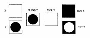
Figure 3.3 Boolean operations on binary images.
3.4 Matrix Operations
Many imaging techniques require that the image be treated as a matrix. In the previous sections we applied operations from pixel to corresponding pixel in the image equation. If the operation is addition or subtraction, the matrix operations are identical.
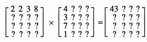
However, if the operation is multiplication, the method discussed in Section 3.2 is called the dot product. The dot product is often used to correct for sensor array response problems where a calibration image is generated for which each pixel value is calculated as a multiplicative correction factor. Images acquired by the sensor can be multiplied by the calibration image to remove or attenuate the individual pixel discrepancies and make the image consistent across all pixels. However, when discussing matrix operations, multiplication of images is normally understood to be the cross product, or vector product. The cross product of two images is substantially different from the dot product and requires an understanding of vector multiplication. Think of a vector as being a single vertical line (a row vector) or horizontal column (a column vector) of an image. Profiling is the process of examining or extracting a vector from an image. Multiplication of a row vector with a column vector results in a scalar, or single-dimensional number. The reason for this is because of the mathematical definition of vector multiplication and we need not explore it further. It is only important here that we understand how it is done. Consider the following example:
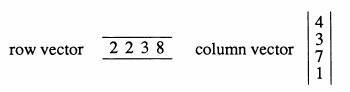
For vector multiplication, we take the corresponding elements of each vector as we go from left to right on the row vector and top to bottom on the column vector. We then add each of the sums to obtain the result, which is (2 x 4) + (2 x 3) + (3 x7) + (8 x 1) = 43. If we wish to take the cross product of two images, i.e., the matrix multiplication, we multiply each of the row vectors of the first image by each column vector in the second. Both images must have the same spatial resolution, or dimension, both horizontally and vertically. If the images are 4 by 4, then we will have 16 values after the calculations, and these values are the pixels of the resulting image. For example,
The first row of the first image multiplies the first column of the second image to yield the first element of the result image under vector multiplication. Note the index for the result is [1, 1]. The index of each element in the result image tells us which row-column pair to multiply to get the value for that pixel. To get the value of the [3, 4] pixel, we would vector multiply the third row of the first image with the fourth column of the second image. A code sample is given of a function that cross multiplies two images that we will call cross_multiply. The function accesses global matrix variables containing the images (X and Y) and storing the result (Z).