Dynamic Texture Recognition

Payam Saisan, Gianfranco Doretto, Ying Nian Wu, Stefano Soatto
Èñòî÷íèê: www.vision.cs.ucla.eduzSzpaperszSz487_doreetto.pdf/saisan01dynamic.pdf

Abstract

Dynamic textures are sequences of images that exhibit some form of temporal stationarity, such as waves, steam, and foliage. We pose the problem of recognizing and classifying dynamic textures in the space of dynamical systems where each dynamic texture is uniquely represented. Since the space is non-linear, a distance between models must be defined. We examine three different distances in the space of autoregressive models and assess their power.

1. Introduction

Recognition of objects based on their images is one of the central problems in modern Computer Vision. We consider objects as being described by their geometric, photometric and dynamic properties. While a vast literature exists on recognition based on geometry and photometry, less has been said about recognizing scenes based upon their dynamics. In this paper we consider the problem of recognizing a sequence of images based upon a joint photometric dynamic model. This allows us to recognize not just steam from foliage, but fast turbulent steam from haze, or to detect the presence of strong winds by looking at trees.

We represent images of stationary processes as the output of a stochastic dynamical model. The model is learned from the data, and recognition is performed in the space of models. The implementation of this idea, however, is not simple. First, the map from a sequence to a model is not necessarily one-to-one: very different scenes can be output of the same model. Second, even the simplest linear models learned from data represent equivalence classes of statistics: the same scene can result in very different models depending on the initial condition. Recognition in the space of models amounts to doing statistics on quotient spaces that have a non-trivial Riemannian structure.

Recognition of complex motion patterns in images is an active area of research in computer vision. Extensive work has been conducted for the case of human motion and in particular facial expressions, for instance [2, 8, 3, 16, 13]. Some methods are based on optical flow. For each frame the flow can be approximated with a small-dimensional vector in a suitable basis, as in [7], and the recognition is done with hidden Markov models (HMMs), or, as in [2], a spatio-temporal representation of the optical flow can be built. Others look at different spatio-temporal features [12].

In this paper we take a different approach: we do not choose local features, nor do we compute optical flow. Instead, we start from the assumption that the sequences of images are realizations of second-order stationary stochastic processes (the covariance is finite and shift-invariant). We set out to classify and recognize not individual realizations, but statistical models that generate them. This entails choosing a distance between models. This problem has been first addressed by Martin in [11], where a distance for single-input, single-output (SISO) linear Gaussian processes has been introduced. We propose and analyze three distances. The first uses principal angles between specific subspaces derived from AR1 models. The second is the extension of the distance proposed by Martin. Both draw on recent results of De Cock and DeMoor [4]. Finally, we also look at the geodesic distance.

2. From image sequences to dynamical models

We start from the assumption that a sequence of images is a realization of a second-order stationary stochastic process. This means that the joint statistics between two time instants is shift-invariant. Although this may seem like a severely restrictive assumption, it has been shown in [14, 6] that sequences such as foliage, water, smoke, and steam are well captured by this model. These sequences are called "dynamic textures".

It is well known that a positive-definite covariance sequence with rational spectrum corresponds to an equivalence class of second-order stationary processes [10]. It is then possible to choose as a representative of each class a Gauss-Markov model - that is the output of a linear dynamical system driven by white, zero-mean Gaussian noise - with the given covariance. In other words, we can assume that there exists a positive integer n a process {x(t)} (the "state") with initial condition and a symmetric positive semi-definite matrix

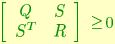
such that {y(t)} is the output of the following Gauss-Markov "ARMA" model2: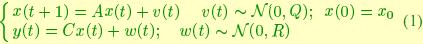

for some matrices and .

While there are many possible choices of canonical realizations (see [9]), we are interested in one that is "tailored" to the data. Since we work with images, we will make the following assumptions about the model (1):

and choose a realization that makes the columns of F orthonormal:

This guaranties that the matrix C is an element in the Stiefel manifold V(m,n) (the set of n orthonormal vectors in Rm) and that the stochastic realization corresponding to a given dataset is uniquely determined. We shall see that the classification/recognition problem can be posed by computing statistics on such a manifold.

The problem of going from data to models can be formulated as follows: given measurements of a sample path of the process: 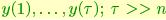estimate a canonical realization of the process {y(t)}. As described in [14], the choice of results in a canonical realization. Ideally, we would want the maximum likelihood solution from the finite sample, that is the argument of

Notice that we do not model the covariance of the measurement noise since that carries no information on the underlying process. In practice, for reasons of computational efficiency, we settle for a suboptimal solution described in [14]. From this point on, therefore, we will assume that we have available - for each sample sequence - a model in the form {A,C,Q}. For the purpose of recognition, we consider processes with different input noise covariance as equivalent. Therefore, the problem of recognizing dynamic textures can be posed as the problem of recognizing pairs {A,C}estimated from data.

2.1. Geometric structure of the space of models

Models, learned from data as described in the previous section, do not live in a linear space. While the matrix A is only constrained to be stable (eigenvalues within the unit circle), the matrix C has non-trivial geometric structure for its columns form an orthogonal set. Let 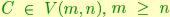be a point on the Stiefel manifold of n-frames in endowed with the Euclidean metric where the tangent plane to the Stiefel manifold. It is shown in [5] that geodesic trajectories in V(m,n) have the general form

and is a skew-symmetric matrix having blocks

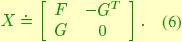
Note that X belongs to a linear space that is isomorphic to , and could therefore be used as a local coordinatization of the Stiefel manifold V(m,n). We will use the structure of the geodesic in order to define a distance in V(m,n) as follows: consider two points and the geodesic connecting them:
and
for a particular value of X, t and for any U, an orthogonal completion of C1. Then we define

where the subscript F indicates the Frobenius norm.

2.2 Probability distributions on Stiefel manifolds

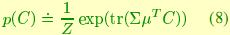
In order to provide a simple statistical description on the space of models, we assume that A and C are independent, so that their statistical description can be addressed separately. While specifying a probability density in the space of transition matrices A is straightforward (indeed, we will adopt a Gaussian density), doing so for the output matrices C is not trivial since, as we have just seen, the space has a non-trivial curvature. In this paragraph we introduce a class of probability densities on the Stiefel manifold that can be used to model the statistics of C. Consider the following function p:

where and where 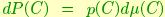with the base (Haar) measuró on V(m,n). We call this function a Langevin (or Gibbs) density on V(m,n), owing to its similarity to Langevin distributions on the sphere. plays the role of the mode of the density, and plays the role of the dispersion. It is easy to verify that the above density has a unique maximum for The functional expression of p can be used to compute likelihood ratios for recognition once the parameters have been inferred.

In order to estimate the sufficient statistics from samples, let 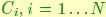be a fair sample from the density p(C). It follows from the law of large numbers that

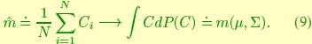
Having a closed-form expression of the integral , one could use samples to compute and use the equation above to compute statistics. However, we do not pursue that avenue further here. Instead, we consider the maximum likelihood estimation of the sufficient statistics by considering the joint density of a fair sample 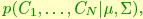which can be written as

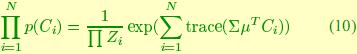
For example, for the case we can look for that solves the following problem

Letting be a singular value decomposition, then

This also clarifies the relationship between the sample mean and the sample median : the latter consists of the orthogonal factors of the former, or in other words it is the orthogonal projection of onto V(m,n).

3. Recognizing dynamical models

As we have articulated in the previous section, a dynamic texture is described by a linear dynamical system and represented by the matrices A,C,Q. This space has a non-trivial curvature structure that must be taken into account when doing statistics or comparisons between models.

In this section we consider three approaches to recognition. One involves computing likelihood ratios, with an explicit form for the probability density of the models. The second involves computing angles between subspaces of the measurement span. The third only involves computing distances between models.

Suppose that two groups of points on V(m,n) are given: , fair samples from a Langevin distribution with mean and dispersion , and samples from a distribution with mean and dispersion . Given a new point C, we want to decide to which "group" it belongs. From a decision-theoretic point of view, the goal is to construct a density corresponding to each hypothesis, 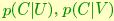, and to compute the likelihood ratio

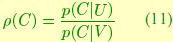
where the parameters and in are computed from the samples as above, and so for and . A decision can then be made based on whether the ratio is larger or smaller than one. This setting can be generalized to decisions among a number of hypotheses in a straightforward fashion [15].

While included in the discussion, likelihood ratios were not part of our experimental scheme. In our experiments we focused mainly on subspace angles and distances between models.

Let and be two matrices with full column rank. The principal angles between range(A) and range(B) are defined as

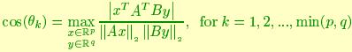
Subspace angles are the largest of these angles. A closed form solution is presented in [4]. We use subspace angles between dynamic texture models to compute distances.

For the sake of simplicity in our implementations we assumed to be dealing with AR models. So, we discuss and compute principal angles and Martin distances between AR models defined by {A,C} pairs. While this assumption may seem restrictive, the results are nonetheless encouraging (see Section 4.2).