Библиотека

Тематическая статья №1

Critical Path Tracing - an Alternative to Fault Simulation

M. Abramovici, P.R. Menon, D.T. Miller

Critical Path Tracing - An Alternative to Fault Simulation. Bell Laboratories, Naperville; 27-29 June 1983. On page(s): 214- 220

Abstract

We present an alternative to fault simulation, referred to as critical path tracing, that determines the faults detected by a set of tests using a backtracing algorithm starting at the primary outputs of a circuit. Critical path tracing is an approximate method, but the approximations introduced occur seldom and do not affect its usefulness. This method is more efficient than conventional fault simulation.

1. Introduction

Fault simulation is performed for the following applications:
• grade a test by determining its fault coverage;
• construct a fault dictionary;
• in the context of test generation, determine a yet undetected fault as the next target for test generation;
• post-test diagnosis.

There are three general methods for fault simulation, namely parallel, deductive, and concurrent. In addition, two other methods deal only with combinational circuits, namely single fault propagation and Hong's method. A combination of these two techniques is used in the PODEM-X test generation system. Specialized methods for combinational circuits are justified by the widespread use of design for testability techniques, such as LSSD, that transform a sequential circuit into a combinational one for testing purposes. Even for combinational circuits, the time spent in fault simulation alone is proportional to n 2, where n is the number of gates in the circuit. The increase in the gate count in VLSI circuits requires more efficient methods for test evaluation and test generation.

In this paper we present an alternative to fault simulation, referred to as critical path tracing. It consists of simulating the fault-free circuit (true-value simulation) and using the computed signal values for tracing paths from primary outputs (POs) towards primary inputs (PIs) to determine the detected faults. Compared with conventional fault simulation, the distinctive features of critical path tracing are:
• it directly identifies the faults detected by a test, without simulating the set of all possible faults. Hence all the work involved in propagating the faults that are not detected by a test towards the POs is avoided.
• it deals with faults only implicitly. Therefore we no longer need fault enumeration, fault collapsing, fault partitioning (for multipass simulation), fault insertion and fault dropping.
• it is based on a path tracing algorithm that does not require computing values in the faulty circuits by gate evaluations or fault list processing
• it is an approximate method.

Consequently, critical path tracing is faster and requires less memory than conventional fault simulation. The approximation occurs seldom and consists in not marking as detected some faults that are actually detected by the evaluated test. We shall show later that this approximation does not affect the usefulness of the method.

Critical path tracing can be extended to synchronous sequential circuits using an iterative array model. In this paper we will restrict ourselves to combinational circuits.

2. Main concepts

Definition 1: A line l has a critical value v in the test (vector) t iff t detects the fault I s-a-v. A line with a critical value in t is said to be critical in t.

Note that unlike the D notation of the D-Algorithm, a critical value always indicates the detection of a fault.

Clearly, the POs are critical in any test. Our test evaluation method consists of determining paths of critical lines, called critical paths, by a backtracing process starting at the POs. Finding the critical lines in a test t, we immediately know the faults detected by t.

Definition 2: A gate input i is sensitive if complementing the value of i changes the value of the gate output.

Critical path tracing starts after the true-value simulation of the circuit for a test t has be.on performed. To aid the backtracing, we mark the sensitive gate inputs during the true-value simulation. The sensitive inputs of a unate gate with two or more inputs are easily determined as follows:
1) if only one input i has a Dominant Logic Value (DLV), then i is sensitive. (AND and NAND have DLV 0; OR and NOR have DLV 1)
2) if all inputs have value not-DLV, then all inputs are sensitive,
3) otherwise no input is sensitive.

The marking of the sensitive gate inputs during true-value simulation involves little overhead, since scanning the gate inputs for DLVs is inherent in commonly used methods for gate evaluation.

First we illustrate critical path tracing in a fanout-free circuit, using the example in Figure 1. Figure la shows the results of true-value simulation with the sensitive inputs marked by dots. Figure l b shows the critical paths by heavy lines. For a fanout-free circuit (which always has a tree structure), critical path tracing is a simple tree traversal procedure that marks as critical and recursively follows in turn every sensitive input of a gate with critical output. This is based on the obvious fact that if a gate output is critical, then its sensitive inputs, if any, are also critical. For the example in Figure 1, note how critical path tracing completely ignores the part of the circuit bordered by the lines B and C, since working backwards from the PO it first determines that B and C are not critical.

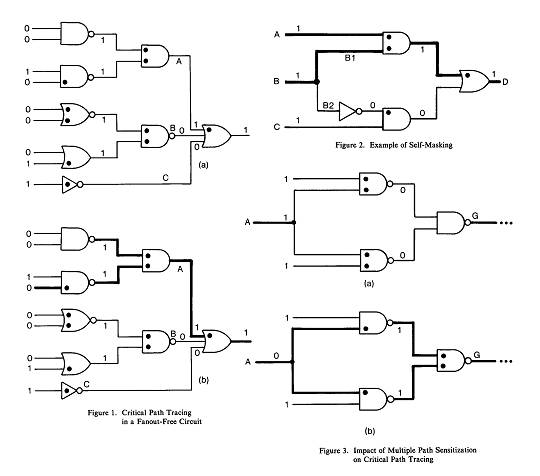
Now we shall discuss the general case of a circuit with reconvergent fanout. Under the stuck fault model, for a signal with fanout we distinguish between its stem and its fanout branches (FOBs). For example, in Figure 2 the lines BI and B2 are FOBs of the stem B. The difficulty in extending critical path tracing to circuits with reconvergent fanout is determining when a stem is critical, given that at least one of its FOBs is critical. In Figure 2 we cannot extend the critical path from BI to B because the effects of the fault B s-a-O propagate on two paths with different inversion parities such that they cancel each other when reconverging at the gate D. This phenomenon is referred to as self-masking.

Following Hong's approach, we separate the test evaluation problem into two subproblems: one deals with fanout-free regions (FFRs) of the circuit, and the other with stems. The strategy adopted in is to first determine the detectability of the stem faults by explicit fault simulation, then trace critical paths in every FFR whose stem fault has been detected. This mixed strategy represents an improvement compared with the explicit simulation of all faults. Our strategy is to determine detectability of the stem faults as they are reached during backtracing by a novel type of analysis that, as we will show later, is much more efficient than their explicit fault simulation. This analysis is described in the next section.

Another effect of reconvergent fanout is that faults that are detected only by multiple-path sensitization may be declared to be undetected, as illustrated in Figure 3a. Here none of the inputs of the gate G is critical, but the fault on A is detected by double path sensitization. As critical path tracing involves establishing unbroken chains of critical lines, it will not recognize the stem A as critical in that test; therefore it is only an approximate method. We shall discuss the implications of this approximation in Section 4.

Note that the case when multiple paths are sensitized from a stem such that we have not-DLV values at a reconvergence gate [see Figure 3(b)] does not pose any problem for our method.

3. Algorithm for Critical Path Tracing

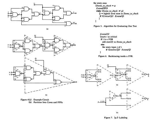
First we preprocess the circuit to determine its cones, where a cone is the subcircuit feeding one PO. We represent a cone as an interconnection of FFRs. Figure 4(b) shows these structures for the adder in Figure 4(a). The inputs of a FFR are FOBs and/or PIs. The output of a FFR is either a PO or a stem. Note that whether a line i is a stem may depend on the cone containing it. For example, N and CI are stems in the cone of S, but not in the cone of CO. Constructing cones and FFRs is commonly done as a preprocessing step in test generation for LSSD circuits.

Figure 5 outlines the algorithm for evaluating a given test. It assumes that true-value simulation, including the marking of the sensitive gate inputs, has been performed. The algorithm processes every cone starting at its PO and alternates between two main operations: critical path tracing inside a FFR, represented by the procedure Extend, and checking a stem for criticality, done by the procedure Critical. Once a stern j is found to be critical, critical path tracing continues from j.

Figure 6 shows the recursive procedure Extend(i) that backtraces all the critical paths inside a FFR starting from a given critical line i by following lines marked as sensitive. Extend stops at FFR inputs and collects all the stems reached in the set Stems to check.

Every stem in Stems to check has at least one critical FOB. The algorithm always selects the highest level stem for analysis (i.e., the closest to the PO), and hence guarantees that the status (critical/non-critical) of all its FOBs is known. The key element in the algorithm is the routine Critical (j) that determines whether the stem j is critical.

To determine the criticality of a stem, we will find out whether self-masking occurs.

A Simple Case.
First we will show a simple preprocessing technique that allows us to directly identify some stems as critical without any analysis. When a cone is built by topological backtracing starting from its PO, with every FFR input and output i we associate a label (v,l) defined as follows.

Definition 3: A line i has a label (p,l) if all paths from i to the PO of the cone pass through 1, and every path from i to I has parity p.

Figure 7(a) shows the (p,l) labels in the cone of S. Clearly all inputs of a FFR get the same I. If all the FOBs of a stem j have the same (p,l) label, then this is assigned to the stem; otherwise j is assigned the label (0,j). The following lemma allows us to mark stems as critical without additional analysis.

Lemma 1: If the label of a stem j is (p,l), where l<>j, then whenever j is reached by backtracing it can always be marked as critical.

Proof: Line j can be reached during backtracing only if l has already been proved to be critical. Since all the paths from j to l have the same parity, self-masking cannot occur between j and I. Hence the fault on j propagates to 1, and because l is critical, it also propagates to the PO. Therefore j is also critical.

Figure7(a) shows the (D,l) labels for the S cone of Figure4: According to Lemma 1, Critical will immediately return TRUE for the stems L and T. Note that the labeling is done per cone, as L has to be checked for criticality in the cone of CO. In our example, both L and T have all their FOBs feeding the same FFR; Figure 7(b) shows a different situation in which a stem (P) need not be checked.

General Case.
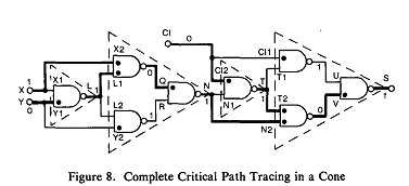
To illustrate the principle used by Critical (j) to check a stem j that does not satisfy Lemma 1, consider the cone of S for the test (X,Y, CI) = 100 (see Figure8). After performing Extend(S), we determine that T2 and N2 are critical. At this point Stems_to_check = {T,N}. Critical(T) returns TRUE immediately and Extend(T) flags CI2 as critical. Now Stems to check = {N, C1} and N is selected for analysis. For the purpose of explanation only, suppose we insert a s-a-O fault on N. The effects of this fault start propagating along two paths, one starting at the critical FOB (N2), and the other at the non-critical one (N1). Self-masking may occur only if the propagation along the latter path, referred to as potentially masking, "kills" the propagation along the critical path as illustrated in Figure 2. It is easy to determine that this type of reconvergence does not occur in Figure 8, since the potentially masking path is immediately stopped at the gate T, as it enters the gate via an input not marked as sensitive. Hence we can immediately conclude that N is critical. We emphasize that propagation along the critical path beyond N2 is not needed because we have determined that all the potentially masking fault effects have disappeared. This is similar to the concepts used in single fault propagation.

The Algorithm.
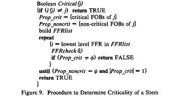
Figure 9 outlines the procedure Critical(j). First it examines the (p,l) label of the stem j to determine whether it satisfies Lemma 1. If not, the check for the criticality of j implicitly keeps track of the propagation of the fault effects of j along critical paths versus propagation on potentially masking paths. The two propagation frontiers are maintained in the sets Prop_crit and Prop_noncrit. These sets consist only of FOBs and stems. FFRlist is the set of FFRs directly fed by the FOBs in Propcrit and Prop_noncrit. The algorithm always selects the lowest level FFR from FFRlist for checking, and hence it guarantees that the status of all the FFR inputs with respect to the propagation of the fault on j is known. The procedure FFRcheck (i) determines the propagation of the two frontiers through FFR i; hence it implicitly determines whether the fault effects arriving on FFR inputs reach its output. The salient feature of FFRcheck (i) is that it usually "jumps" from the inputs of FFR i directly to its output without tracing through any gate inside the FFR. The following example illustrates different cases of FFR jumping. (A detailed description of the algorithm is beyond the scope of this paper.)

Example.
Suppose that the lines currently identified as critical are those shown in Figure 10 and now the problem is to determine whether A is critical. The table traces the execution of Critical(A).

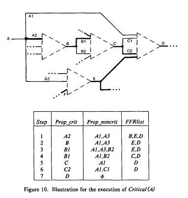
Step 1: Starting with Prop_crit={A2} and Prop_noncrit={A1,A3}, the first FFR checked is B, which is reached only by lines in Prop_.crit (A2). Here no masking can occur inside the FFR, hence the fault effect on A2 propagates on B; therefore we add B to Prop_crit.

Step 2: The FOBs of B (B1 and B2) are added to the two frontiers based on their previously determined criticalities.

Step 3: Next we analyze FFR E, which is reached only by one line in Prop_noncrit (A3). Since E has a critical input (F), the propagation from A3 to E is bound to stop inside the FFR. The reason is that there must exist a gate G where the path from A3 will converge with the critical path from F, such that the critical input of G has a DLV.

Step 4: FFR C is reached by lines in both frontiers - BI in in Prop_.crit and B2 in Prop_noncrit. But the propagation from B2 cannot stop the propagation from B1, because the algorithm had already determined this when it established that B was critical. Therefore we add C to Prop_crit.

Step 5: The FOBs of C are added to the two frontiers.

Step 6: The criterion we used to skip FFR C cannot be used to skip FFR D, because of the additional potentially masking line reaching it (AI); A1 did not play any role in determining the criticality of C. Now we apply a different criterion to avoid tracing inside the FFR. Let p (A1), p (C1), p (C2) denote, respectively, the inversion parities between A1, C1, and C2, and D. Let v(A1), v(C1) and v(C2) be their current values. It can be shown that if v(AI) XOR p(A1)=v(CI) XOR p(Cl)=v(C2) XOR p(C2), then masking cannot occur inside the FFR D. Assuming that this relation is satisfied in Figure 10(a), we add D to Prop crit.

Step 7: At this point Prop noncrit=0 and |Prop__crit|=1 (since Prop_crit={D}); hence the procedure returns identifying A as critical.

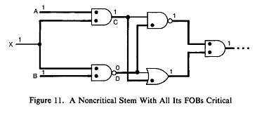
One may wonder why the condition Prop_noncrit=~b alone is not suflq.cient for stopping the forward tracing. The answer is provided by the example in Figure 11, which shows a stem (X), all of whose FOBs are critical (hence Prop_nonerit=0). However, contrary to one's intuition, X is not critical. The reason is that the potentially masking lines appear after propagation through C and D. Requiring |Prop__crit|=l and Prop_noncrit=0 guarantees that no masking can further occur.

If none of the "FFR jumping" criteria applies, then path tracing proceeds inside a FFR. This is similar to the path tracing at the FFR level, i.e., propagating the frontiers Prop_crit and Prop_noncrit in a breadth-first manner. Note that no gate evaluations are involved, and even the gate types and the signal values are unnecessary for this analysis; the only information needed is provided by the sensitive markings.

We emphasize that in most cases self-masking does not occur and the propagation of the potentially masking fault effects is "short-lived"; therefore, little effort is usually needed to determine that a stem is critical.

Our method consists of the following steps: (1) Preprocessing the circuit model, to determine its cones and FFR structure and the (p,l) labels. (2) True value simulation of one test and identification of the sensitive gate inputs. (3) Critical Path Tracing, which is a backtracing procedure that identifies the critical lines (and hence the detected faults) in the test simulated in step 2. Steps 2 and 3 are repeated for every test in the set of tests under evaluation.

4. Conclusions

The key factors contributing to the increased efficiency of critical path tracing compared to fault simulation are as follows:
• it deals directly only with the detected faults rather than all possible faults,
• it deals with faults only implicitly rather than explicitly,
• it is an approximate rather than an exact technique.

The approximation introduced is pessimistic and consists in not marking as detected some faults detected by multiple path sensitization with DLVs at a reconvergence gate. This phenomenon occurs seldom. However, we have shown that the approximation does not affect the test generation process and has practically no impact on the other applications of critical path tracing.

The advantages of test evaluation by critical path tracing over conventional methods strongly suggest that solutions to the VLSI testing problems should be based on approximate algorithms that are fast and generally accurate. A gain of one order of magnitude in execution time is much more important than an "exact" algorithm whose only advantage is that it is capable of correctly processing situations that occur seldom. Furthermore, one can question the wisdom of using exact and costly algorithms for an approximate fault model.