To develop a neural network, which will predict the financial and economic indicators, such problems are solved: selection of
input and output data, network topology, learning method of neural network activation function. Time series of price will be
enough to make an accurate prediction. It is divided into three sets: training, testing and control samples, which are fed
to the inputs of the network.
Pretreatment data is an important step in the application of neural networks trained with the teacher and determines the
learning rate, the value of training and generalization errors and other properties of the network. There most commonly used
linear shift of the interval characteristic value, for example, in the interval [-1,1] for the preprocessing of quantitative
variables. Formula for converting the characteristic value x for the i-th sample cases in the interval [a, b] is:

where xmin , xmaxare minimum and maximum sample values of the trait. In the absence of severe
restrictions on the range of the preprocessed feature scaling can be accomplished, which gives zero mean and unit variance
preprocessed value, according to the formula:

where M(x),σ(x) - are the original sample mean and standard deviation. Getting a zero average for the input network
speeds up a gradient learning, because it reduces the ratio of maximum and minimum matrix’s non-zero values of objective
function’s second derivatives of network settings. [1]
As the topology of the neural network is proposed multi-layer perceptron, as it shows on average the best results in problems of time series prediction.
In this topology, neurons are regular organized in layers. The input layer consisting of sensitive (sensory) S-element, which receives input signals Xi,
does not commit no processing of information and performs a distribution function. Each S-element associated with a set of associative elements (A elements)
of the first intermediate layer, and A-elements of the last layer are connected to the responder (R-elements).
 Figure 1. Structure of multilayer perceptron(animation: 5 frames, delay 0.4 sec, weight 28.6 kB)
Weighted combination of outputs R-elements make up the reaction system, which indicates that the object is recognized in certain way. If there are being
recognized only two images, then the perceptron sets one R-element, which has two reactions - positive and negative. If there are more than two images, then
for each image is determined it’s R-element, and the output of each element is a linear combination of outputs A-elements. [2]
As a method of training the neural network was chosen the method of back-propagation errors. The basic idea of back propagation is to get an assessment
of error for the neurons of hidden layers. Note that the known bugs, a submission by the neurons of output layer, are caused by unknown errors neurons of
hidden layers yet. The higher the value of synaptic connections between neurons of the hidden layer and output neurons, the stronger the error of the first
influences the error of the second. Consequently, the assessment of errors in the elements of hidden layers can be obtained as the weighted sum of errors of
the subsequent layers. While training information is circulating from the lower layers of hierarchy to the highest, and evaluation of errors that make network
is circulating in the opposite direction [3].
At the stage of training synaptic coefficients w are evaluated. However, in contrast to the classical methods it is based on non analytical calculations,
and methods of training samples using the examples are grouped in the training set. For each image from the training sample is known desired output of neural
network. This process can be viewed as a solution to the optimization problem. Its goal is to minimize the error functions or residual E on the training set
by selecting values of synoptic factors w.

where di is a required (desired) output value for the j-th pattern of the sample;
yi is the real value;
p is the number of patterns of the training sample.
Minimizing the error E is usually carried out using gradient methods. Сhanging weights occurs in the direction opposite to the greatest slope of the function error.

where 0 < &eta &le 1 is a user-defined parameter.
There are two approaches to the learning. The first of these weights w are recalculated after the filing of all training set, and the error has the form

In the second approach, the error is recalculated after each sample:


Suppose, that

, so

Then

, where yj(Sj)is an activation function. For


The third factor is:

One can show that

while the summation k is among the neurons of the n-th layer.We introduce a new notation:

For an internal neuron:

For an outside of the neuron:


Thus, a complete back-propagation learning algorithm is constructed as follows:
1. Feed to the inputs of the network one of the possible samples in the normal operation mode of the neuron network, when the signals propagate from the inputs
to the outputs to calculate the yields of all neurons (usually the initial values of the weights are small).
2. Calculate the values of &delta jn for the neurons of output layer according to the formula (13)
3. Calculate the values of &delta jn for all the internal neurons according to the formula (12)
4. Using formula (14) for all links to find the increments of weighting coefficients &Delta W jn.
5. Adjust the synaptic weights:

6. Repeat steps 1-5 for each image of a training set until the error E does not become small enough.
As the activation function of the input and output layers is chosen linear function.

The neurons of hidden layers will be activated by means of rational sigmoid function.

The effectiveness of this variant is determined by the fact that this function is strictly monotonically increasing, continuous and differentiable and the computation
of rational sigmoid compared to the other takes less CPU time.
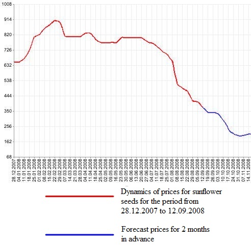
 Figure 2. Schedule of forecasting time series
After selecting a general structure it is necessary to find experimentally the network settings. Network is needed to find the number of layers and the number of neurons
in each of them for. While choosing the number of layers and neurons in them, it is bear in mind that the ability of the network is higher, the greater the total number of
connections between neurons is. On the other hand, the number of connections is bounded above by the number of records in the training data.
Based on the results obtained by experimental means, as a result of the proposed neural network package MatLab, it is obvious that the topology of neural network and
its method of training is very effective in forecasting problems.


