
Abstract
Content
- Introduction
- 1. The purpose of the work
- 2. The essence of the method
- 3. Criteria for evaluating the sign of the roots of a characteristic equation
- 4. Static stability evaluation software
- 5. Evaluation of root sign using algebraic criteria
- 6. An example study of the SU of a proportional-type controlled ARV system
- Conclusions
- References
Introduction
Static stability (CS), or the stability of a steady state, is the ability of an electrical system to return to its original position after a small disturbance (deviation of operating parameters) [1].
In any electrical system, a steady state does not mean the constancy of all its parameters. The electrical system has a large number of loads that change, and these changes appear and disappear. In this connection, some additional insignificant moments appear on the generators of the system, also stochastically, which reduce or increase the moments that act on the shafts of the generators and shift their rotors by small angles [6].
Thus, small disturbances constantly occur in the electrical system, the cause of which and the city of origin are not fixed. These are some free disturbances that cause free movement, which can be growing or decaying, oscillatory or aperiodic. Its nature determines the static stability, which is a necessary condition for operability system. Static stability is checked in prospective and detailed design, development of special automatic control devices (calculations and experiments), commissioning of new system elements, changing operating conditions [7].
Studies of static stability are presented in terms of solving problems of analysis or synthesis.
When solving the problems of analysis, the stability of the mode that has been established is checked, the extremely stable mode of the electrical system specified by all parameters is determined, some quality indicators of the transition process are evaluated.
When solving synthesis problems, the type of the excitation system and its regulation, the law of regulation, the parameters of the excitation system and regulators are determined. At the same time, they proceed from the set requirements for the extremely stable regime or the quality of electricity in the established mode.
The task of determining the conditions of static stability and the nature of transients is quite complicated for real electrical systems that have automatic excitation and speed controllers. To facilitate the solution of this problem, various mathematical techniques and methods are used. One of the most common methods for studying static stability is the method of small oscillations using special criteria that evaluate the signs of the real roots, or the real parts of the complex conjugate roots of the characteristic equations, and thus determine the nature of the transition process (PP).
1. Purpose of work
The aim of the master's work is to develop software for the study of control systems of electrical systems of varying complexity by the method of small oscillations using practical algebraic and frequency criteria on a computer.
To achieve this goal, the following tasks will be solved:
- analysis of the theoretical provisions of the study of the static stability of electrical systems using algebraic criteria (Hurwitz, Routh) and frequency criteria (Mikhailova, D-partition);
- software development for the implementation of these methods on a PC;
- development of guidelines for the study of static stability using software.
2. The essence of the method
Perturbations in the system that cause small deviations considered in the study of static stability are not determined not by the place of their occurrence, not by magnitude. That is, the origin of the disturbance is such that it is impossible to establish the absolute values of the regime parameters when they deviate from the established (initial) values. Thus, the task of studying static stability is reduced to the task of determining only the nature of the change in the parameters of the regime.
When establishing practical criteria, the answer was only in the form of a yes-no
, stable-unstable
mode from the initial state with small perturbations. In any case, the nature of the transition process (aperiodic, oscillatory, decaying, growing) will be determined by possibly solving or analyzing a system of nonlinear differential equations.
Russian mathematician it was proved to Lyapunov that static stability can be judged by a linearized system of equations, since small deviations are those in which the system behaves as linear. He proved two theorems, the essence of which lies in the first approximation method (the first Lyapunov method): the system is stable in the small (statically) if its linear approximation is stable.
The method of studying static stability by linearized equations is called the method of small oscillations or small deviations [4]. Linearization is as follows. Any independent variable is also depicted as the sum of a constant in the initial mode and an infinitely small approximation:

By expanding the nonlinear functions into a Taylor series and leaving only the linear terms of this series, we obtain a system of linear differential equations, but with respect to infinitely small increments. The solution to such a system has the form [9], [4]:

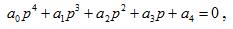
where p – are the roots of the characteristic equation, which in canonical form looks like this:

The number of components is equal to the order of the system of equations. Since the coefficients of the characteristic equation, which are determined by the real parameters of the system, are real numbers, its roots can be real, or complex conjugate. Thus, having compiled a characteristic equation and determining its roots, it is possible to determine the nature of the change in small increments of the regime parameters over time. The real root corresponds to a member of the form  . A pair of complex conjugate roots
  . When all the roots and the real parts of all complex roots are negative, then all the components of the transition process modulo decay exponentially. The observed mode in this case is statically stable. When at least one positive appears among the real roots, the corresponding component of the transition process will grow exponentially unlimitedly. The output mode is statically unstable (aperiodic disturbance of stability or
 sliding
). When a pair having a positive part appears among the complex roots, the corresponding component will have the form of oscillations increasing in time.
Thus, a necessary and sufficient condition for the static stability of the initial mode of the electrical system is the requirement that all real roots and real parts of all complex roots of the characteristic equation be different. There are methods (criteria) that allow you to determine the signs of the roots and thus judge the stability of the system without defining the very roots of the characteristic equation. The order of operations for studying the static stability of electrical systems by the method of small oscillations is as follows [9]:
- Make a mathematical description of transients in the system in the form of nonlinear differential equations.
- The linearization of the original equations is carried out in order to obtain linearized equations.
- There is a characteristic equation and a characteristic determinant.
- Stability is assessed using criteria that provide signs of the roots.
3. Criteria for evaluating the sign of the roots of the characteristic equation
Stability criteria are classified as direct, which require finding the roots, and indirect, which do not require calculations of the roots. These include algebraic (Hurwitz, Route method) and frequency (Mikhailov, Nyquist, D-partitions) methods [9].
4. Static stability assessment software
The program is created in the environment of the mathematical integrated package Mathcad. This is because the integrated package has the ability to combine fragments of various systems with each other, while simultaneously using the built-in features of Windows. These include:
- use of all Windows tools;
- modern multi window interface;
- color paperwork;
- creation of animated dynamic files;
- sound creation.
These systems have a convenient interface - means of communication with the user in the form of windows that move, keys and other elements. They have effective means of scientific graphics. Given that most of the time it takes to prepare the text, it is advisable to work in the environment of the Word text editor, and paste objects with MathCAD [3]. Such an insertion into the word processor of objects from the mathematical system MathCAD gives full access to all the possibilities and means of the latter. It is also possible to use a hyperlink to call a file created in the MathCAD environment. Using special keys when using hyperlinks, you can easily rotate to the previous or next document. Text, formulas and simple drawings (output schemes, equivalent schemes) are generated directly in the Word editor. Illustrations, which are a graphical result of calculations (vector diagrams, functional dependencies, and others) are formed in the MathCAD environment with the subsequent implementation of the resulting figure in a Word document. Animated drawings (rotating vector diagrams and coordinate axes, functions and graphs, as well as a sequence of solution results for various input data, etc.) are also created in the MathCAD environment. To create a sequence of animation frames, the standard technology for creating animation files with the extension “avi” is used. Double-clicking the left mouse button when placing the cursor on a drawing made using the MathCAD system allows you to activate the latter and use its capabilities for analysis, the influence of various factors on the nature of the transition process. If you close the MathCAD window, you will be rotated to the Word document that was studied. Animated drawings can be called directly from a Word document using hyperlinks, or temporarily created in the MathCAD environment. It is possible to perform various kinds of calculations if you call MathCAD documents from a text file, based on existing links, and vice versa, when performing calculations, you can turn to textual material to get the necessary help.
The software (software) for assessing the static stability is developed for the simplest electrical system, which is shown in Fig. 1

Figure 1 – Scheme of the simplest electrical system
(the animation consists of 8 frames with a delay of 500 ms between frames, the number of playback cycles – 3, size – 10 kilobytes)
5. Assessment of the sign of roots using algebraic criteria
Hurwitz criterion.
For a controlled system with proportional-type ARV, strong action, the values of the coefficients of the characteristic equation are as follows [4], [9]:
where

The determinants of Hurwitz and all additional determinants are calculated. For the output, the value of the mentioned Hurwitz determinants is displayed on the monitor screen. The roots of the characteristic equation of the system, which is studied using the means of symbolic mathematics Mathcad, are calculated [3]:
The values of all Hurwitz determinants are compared with the obtained roots of the characteristic equation. Based on this comparison, conclusions are drawn about the conditions of violation of the SU of various types (aperiodic, periodic and self-excitation). The analysis allows you to determine the conditions of stability loss at different values of the gain of the ARV. It is also possible to identify the effect on the ku value of the control time constant. The Hurwitz determinants, all additional determinants and roots of the characteristic equation are also calculated. An analysis of all these parameters is carried out and conclusions are drawn about the conditions of violation of static stability.
Критерий Рауса
For the simplest regulated system with proportional-type ARV, we calculate the coefficients of the table period. Elements of each next timeline are found by the formula [5], [10]:

where k is the column number; i is the line number in which the coefficient is located. The compiled Routh table is displayed. Based on the number of sign changes in the first column, conclusions are drawn about the conditions of violation of SS of various types.
6. An example of a study of the SU of a regulated proportional-type ARV system
In order for the system to operate statically stably at large angles beyond 90, it is necessary to introduce excitation control [8],  It is known that a statically stable system will work under the following condition.

 — minimum necessary gain;
 — maximum allowable gain [2]. The change in the mentioned coefficients depending on the initial load angle is shown in Fig. 2
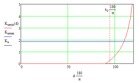
Figure 2 – Change in gain depending on the initial load angle
For the given parameters of the system that is being investigated, the value of the maximum allowable coefficient does not depend on the initial angle and is 1.855. The minimum required ratio depends on the output mode. we see that the system can operate statically stably when a certain gain is introduced.
If  aperiodic stability disturbances will occur in the system. On condition
  self-extracting type.
Consider the example when the system is stable
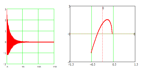
Figure 3 – The nature of the transition process and the hodograph of Mikhailov
An analysis of Fig. 3 shows that for given initial parameters of the regime, the oscillatory process is of a damped nature, which corresponds to a stable system. The hodograph of Mikhailov also corresponds to a stable system.
Conclusions
Thus, the development of software for assessing the static stability of regulated electrical systems, determining the signs of real roots, or the real parts of the complex roots of characteristic equations, graphical interpretation using Mathcad, provides several advantages: visibility, simplicity, the ability to determine stability, without resorting to additional calculations.
At the time of writing, the master's work is not yet complete. Final completion: December 2014. After this date, the full text of the work and materials on the topic can be obtained from the head.
References
- Статическая устойчивость [Электронный ресурс]. – Режим доступа: http://dic.academic.ru.
- Жданов П. С. статическая устойчивость сложныхэлектрических систем. – М.: 1940,
- Дьяконов В. П. : Mathcad 11/12/13 в математике. – Москва
Высшая школа
2007. – С. 315-530. - Переходные электромеханические процессы в электрических системах: Учеб. для электроэнергет. спец. вузов. – 2 – е изд, перераб. и доп. Венников В. А. / М.: Высш. шк, 1970. – 472 с,
- Методы расчета устойчивости энергосиcтем [Электронный ресурс]. – Режим доступа: http://portal.tpu.ru.
- Нелинейная коррекция сильного регулирования возбуждения генераторов. Кощеев Л. А., Невельский В. Л. –
Труды НИИПТ
, 1977, вып. 26. - Ульянов С. А. Электромагнитные переходные процессы. – М.: Энергия, 1970, 518с,
- Статическая устойчивость электрических систем с синхронными машинами, снабженными автоматическими регуляторами возбуждения: Лекции / Розанов М. Н. – М. 1959,
- Переходные электромеханические процессы в электрических системах: Учеб. для электроэнергет. спец. вузов. – 4-е изд., перераб. и доп. Венников В. А. / М.: Высш. шк., 1985. – 536 с.,
- Рюденберг Р., Переходные процессы в электрических системах, изд-во иностранной литературы, 1955.