
Abstract
Content
- Introduction
- 1. Purpose and objectives of the study
- 2. Relevance of the topic
- 3. Domain Analysis
- 3.1 Neural Network
- 3.2 Neuron
- 3.3 Synapse
- 3.4 Activation function
- 3.5 Multilayer Perceptron
- 3.6 Backpropagation
- 3.7 Convolutional Neural Networks
- 4. Overview of research and development
- 4.1. Lalal.ai
- 4.2. Audio editors
- 5. Overview of development tools
- 5.1 TensorFlow and the Keras framework
- 5.1.1 Keras module in TensorFlow 2
- 5.1.2 TensorBoard
- 5.2. PyTorch
- 5.3 ApacheMxnet
- List of sources
Introduction
The problem of audio source separation or audio source separation is quite popular, especially its special case - the separation of music and voice. However, solving such problems with classical algorithms is difficult, especially for voice separation. The algorithms themselves are quite complex, and the result is far from ideal. It should also be borne in mind that there may be several votes, and they, in turn, can be processed with reverbs, delays and other effects.
Therefore, to solve such problems, you should use the already quite popular deep machine learning. The algorithm itself must learn to look for suitable features, and extract them, getting a new audio track.
1. Purpose and objectives of the study
The purpose of this work is to find a suitable architecture and train a deep convolutional neural network, so that she is able to extract the voice from the music at a fairly correct level, with the least amount of extraneous noise. The objectives of the study include comparing the created neural network and similar programs with the original "unmixed" voice different compositions to detect errors in the work of the created program[1][2].
2. Relevance of the topic
Although sound processing is a rather interesting practical task, in the field of deep learning, this topic is not explored as much as working with images or texts. Perhaps the reason is the great complexity of development, because if images and you can work with text right away, then the sound needs to be translated into a suitable data array. Basically, work occurs with frequencies, which requires work with the windowed Fourier transform, or with wavelet transforms. Separating voice and music can be useful for more than just extracting a separate music track for songs that do not have one, but also for processing audio recordings voices, noise reduction, etc. Although there are already many different solutions given a given problem using machine learning, all solutions do not work perfectly. Their work depends on network topology, training sample, error minimization method, and number of iterations. Algorithms are changing, new ones are being developed, therefore, this topic, like many others related to machine training will remain relevant.
3. Domain Analysis
3.1. Neural network
A neural network is a sequence of neurons connected by synapses. The structure of the neural The network came to the world of programming straight from biology. Thanks to this structure, the machine acquires the ability analyze and even memorize various information. Neural networks are also capable of not only analyzing incoming information, but also reproduce it from your memory.
The peculiarity of neural networks lies in their trainability. Neural networks can recognize deeper, sometimes unexpected patterns in the data. In the general sense of the word, learning consists in finding the correct coupling coefficients between neurons (which will be discussed later), as well as in generalizing data and identifying complex dependencies between input and output signals. If at first it is easy to deceive her, then after a couple of hundred thousand actions, she will easily recognize if you trying to give her something wrong.
Most often, for this you need to “run” her work on tens of millions of input data sets, indicating to her the correct and removing incorrect options.
Neural networks are used to solve complex problems that require analytical calculations similar to what does human brain. The most common applications of neural networks are tasks:
• Classifications,
• Predictions,
Let's take a closer look at the main components of a neural network.
3.2. Neuron.
A neuron is a computational unit that receives information, performs simple calculations on it, and passes it on. They are divided into three main types: input, hidden and output. when the neural network consists of a large number of neurons, enter layer term. Accordingly, there is an input layer that receives information, n hidden layers that process it and an output layer, which outputs the result. Each of the neurons has 2 main parameters: input data (input data) and output data (output data). The input field contains the total information of all neurons from the previous layer, after which it is normalized using the activation function.
3.3. Synapse.
A synapse is a connection between two neurons. Synapses have 1 parameter - weight. Thanks to him, the input information changes when transmitted from one neuron to another.
The image below shows part of a neural network, with I representing the input neurons, H representing the hidden neuron, and w representing the weights. It can be seen from the formula that the input is the sum of all the inputs multiplied by their respective weights.
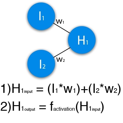
Figure 1 is a schematic representation of the operation of one neuron
Let's input 1 and 0. Let w1=0.4 and w2 = 0.7 The input data of neuron H1 will be the following: 1*0.4+0*0.7=0.4. Now that we have input data, we can get the output by substituting the input value into the activation function.
3.4. Activation function.
An activation function is a way to normalize input (we've talked about this before). That is, if you have a large number at the input, skipping it through the activation function, you will get the output in the range you need. There are a lot of activation functions, so we will consider the most basic ones: Linear, Sigmoid (Logistic) and Hyperbolic tangent. Their main differences are the range of values (Fig. 2-4).
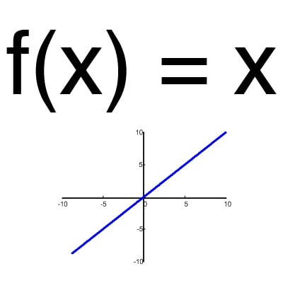
Figure 2 - Linear Function
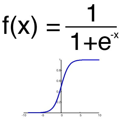
Figure 3 - Sigmoid
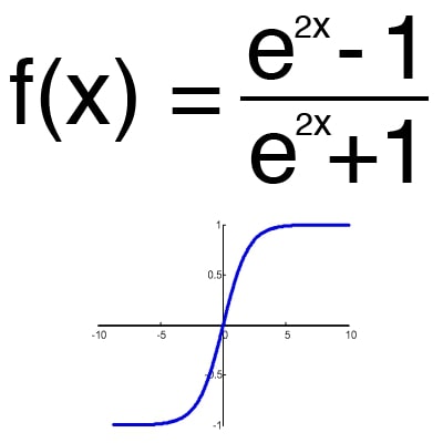
Figure 4 - hyperbolic tangent
3.5. Activation function.
Multilayer perceptron is the simplest and most common neural network. Is a fully connected neural network network (the outputs of the previous layer are connected to all inputs of the next layer) direct propagation (the signal goes only to one side). Each synapse has its own weight, which determines the strength of signal transmission from one particular neuron to another. There can be either several or one output signals, depending on the conditions of the problem[5][6].< /p>
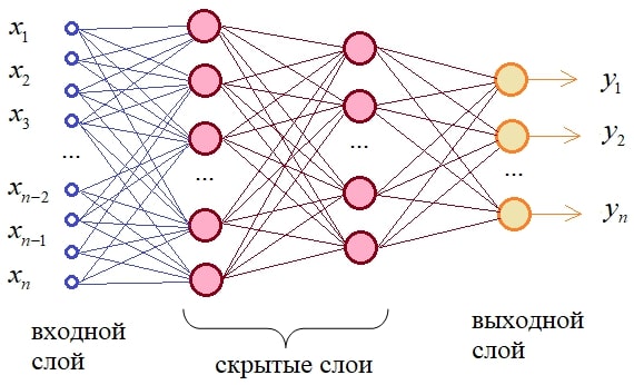
Figure 5 - Schematic representation of a multilayer perceptron
3.6. Backpropagation
To train the neural network from scratch, we take the values of the weights as random numbers from -0.5 to 0.5. Next, you need to check the result of the work, and adjust the weights according to the magnitude of the error. For this, the backpropagation method is used. Backpropagation goals are simple: adjust each weight in proportion to how much it contributes to the overall error. If we iteratively reduce the error of each weight, eventually we will have a series of weights that make good predictions.
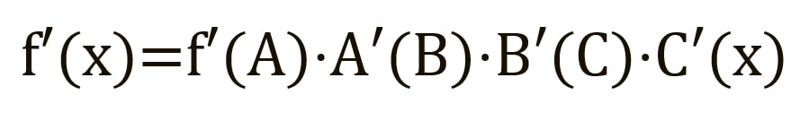
Forward propagation can be thought of as a long series of nested equations. If that's how you think about forward propagation, then reverse propagation is simply an application of the chain rule (differentiation of a complex function) to find derivatives of losses with respect to any variable in the nested equation. Including the direct propagation function:
where A, B, and C are activation functions on different layers. Using the chain rule, we calculate the derivative of f(x) with respect to x:
To find the derivative with respect to B, we can pretend that B (C(x)) is a constant, replace it with a placeholder variable B, and continue searching for the derivative with respect to B in the standard way:
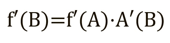
This simple method extends to any variable within a function, and allows us to precisely determine the impact of each variable to the overall result[7][8].
3.7 Convolutional neural networks.
The best results in the field of image analysis were shown by the Convolutional Neural Network or Convolutional Neural Network (hereinafter referred to as CNN). The success is due to the possibility of taking into account the two-dimensional topology of the image, in contrast to the multilayer perceptron.
SNN consists of different types of layers: convolutional layers, subsampling (subsampling) layers and "normal" layers neural network - perceptron, in accordance with Figure 6.
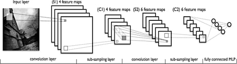
Figure 6 - types of layers in a convolutional neural network
The first two types of layers (convolutional, subsampling), alternating with each other, form the input feature vector for the multilayer perceptron.
The convolutional network got its name from the name of the operation - convolution, the essence of which will be described later.
Determining the network topology is guided by the problem being solved, data from scientific articles and our own experimental experience.
The following steps can be distinguished that affect the choice of topology:
• define the problem to be solved by the neural network (classification, prediction, modification);
• to determine the limitations in the problem being solved (speed, accuracy of the answer);
• define input (type: image, sound, size: 100x100, 30x30, format: RGB, grayscale) and output data (number of classes).
The input layer is a two-dimensional array. The convolutional layer is a set of maps (another name is feature maps, in everyday life it is ordinary matrices), each map has a synaptic nucleus (it is called differently in different sources: a scanning nucleus or a filter).
The number of cards is determined by the requirements for the task, if you take a large number of cards, then the recognition quality will increase, but the computational complexity.
The core is a filter or window that slides over the entire area of the previous map and finds certain features of objects. The core is a system of shared weights or synapses, this is one of the main features of a convolutional neural network.
Initially, the values of each map of the convolutional layer are 0. The weights of the kernels are set randomly in the range from -0.5 to 0.5. The kernel slides over the previous map and performs a convolution operation, which is often used for image processing, the formula:
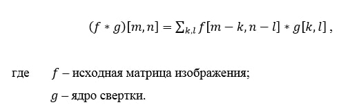
How the convolution operation works
The subsample layer, like the convolutional layer, has maps, but their number is the same as the previous (convolutional) layer, there are 6 of them. The purpose of the layer is reduction of the dimension of the maps of the previous layer. If some features were already identified at the previous convolution operation, then for further processing, such a detailed image is no longer needed, and it is compacted to a less detailed one. Usually, each card has a 2x2 core, which allows you to reduce the previous maps of the convolutional layer by a factor of 2. The entire feature map is divided into cells of 2x2 elements, from which maximum value.
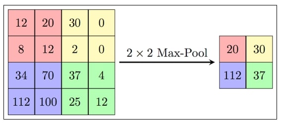
Figure 7 - Generation of a new subsample map based on the previous convolution map. Max Pooling
The last of the layer types is the layer of a conventional multilayer perceptron. The purpose of the layer - classification, models a complex nonlinear function, optimizing which, recognition quality improves[9].
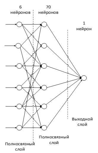
Figure 8 - an example of a fully connected layer in a convolutional neural network
4. Overview of research and development
4.1 Lalal.ai
LALAL.AI is an online service for splitting tracks of any audio format into vocals and music. LALAL.AI analyzes the track and tries to extract information about individual instruments and parts.
The LALAL.AI database contains 20 TB of high-quality studio recordings that are used to train artificial intelligence. This allows the service to cope with the work, making a minimum of errors.
4.2 Audio editors
The separation of music and voice is also supported by many audio editors of varying degrees of quality. The most popular are:
• Audacity.
• Magix sound forge pro.
• FL Studio.
5. Overview of development tools.
5.1 TensorFlow and the Keras framework
Written in C++ by the Google team in 2015, TensorFlow is one of the most popular Deep Learning frameworks. Today we will talk about the interface that provides TensorFlow for Python: the difference between Tensorflow 1 and TensorFlow 2, built-in Keras framework, model building and visualization with TensorBoard.
First of all, we need to draw a line between TensorFlow 1.x and TensorFlow 2.x. They have striking differences. The framework operates static computational graphs, which means that they are only executed at compile time.
5.1.1 Keras module in TensorFlow 2
The Keras deep learning framework has migrated to TensoFlow 2, and its functionality is now stored in the tf.keras module. This module contains model building tools such as:
• Layers, including fully connected (Dense), convolutional (Conv1D), recurrent (RNN, LSTM). There are 105 layers in total;
• Activation functions, including Softmax, ReLU, Sigmoid. Some activation functions, such as PReLU, are available as layers. There are 15 in total;
• Loss functions, including Binary Crossentropy, MAE, MSE. There are 25 in total;
• Metrics, eg MAE, MSE, Cosine Similarity. A total of 43 in the form of classes and 25 in the form of functions;
• Optimizers, including SGD, Adam, Adagrad. There are 9 in total;
• Callbacks, including RemoteMonitor for sending events to the server, History for tracking the history of model events, EarlyStopping for stop the model in case of no improvement, TensorBoard to activate the render mode. There are 14 in total.
5.1.2 TensorBoard
TensorFlow has its own visualization tool, TensorBoard. With TensorBoard you can:
• follow the process of changing accuracy (accuracy) and loss (loss) in real time;
• visualize the model graph with layers and operations;
• show model parameters (weights, blends) or other tensors that change over time;
• display pictures, video or audio;
• and more
5.2. PyTorch
PyTorch, developed by the Facebook team in 2017, is a deep learning framework built primarily for Python.
Unlike TensorFlow, the PyTorch framework does not impose its interface on the developer. You can create your own layers activation functions and other necessary objects in the form of ordinary Python classes and functions. Operations on tensors can be performed on the GPU.
PyTorch uses automatic differentiation for gradient calculations, which are used in the backpropagation algorithm errors (backpropagation). The advantage of this approach is the speed of calculation.
PyTorch not only allows you to work with tensors, but also provides a number of opportunities for deep learning (Deep Learning). PyTorch has four main components required to build models:
• nn is used to create computational graphs that form layers of neural networks (neural net). Similar function in TensorFlow, the Keras module executes.
• optim contains various optimization algorithms (SGD, Adam, etc.). An analogue in TensorFlow is the optimizers module.
• Dataset — interface for representing input and output data in different formats, for example, in the form of tensors (TensorDataset), iterable(IterableDataset) etc. TensorFlow also has a Dataset class.
• The DataLoader converts the Dataset into a manipulated format that can be used to control the batch size, mix data, distribute processes, etc. In TensorFlow, the data module is responsible for this.
To create layers, for example, convolutional (convolutional), fully-conected (fully-conected), recurrent (recurrent), you can use torch.nn module, and for optimization algorithms - torch.optim. However, the model building and training interface is not as high-level as compared to with TensorFlow, so you have to write additional Python code.
5.3. ApacheMxnet
Apache MXNet is an open source deep learning framework used to build, train and deploy deep neural networks. MXNet abstracts the complexities involved in implementing neural networks, has high performance and scalability, and offers API for popular programming languages such as Python, C++, Clojure, Java, Julia, R, Scala and more.
MXNet includes a Gluon interface that allows developers of all skill levels to get started with deep learning technologies in the cloud, at the edge devices and mobile applications. With just a few lines of Gluon code, you can create linear regressions, convolutional networks, and recurrent networks with Long Short Term Memory (LSTM) for object detection, speech recognition, recommendations and customization.
Benefits:
• Easy to use with the gluon interface. The Gluon MXNet library provides a high-level interface that allows easy prototyping, train and deploy deep learning models without sacrificing learning rate. Gluon offers high-level abstractions for predefined layers, functions losses and optimizers. It also provides a flexible framework that is intuitive to use and easy to debug.
• Improved performance. Deep learning workloads can be distributed across multiple GPUs in an almost linear fashion. scalability, which means that even very large projects can be handled in less time. Scaling is performed automatically depending on on the number of GPUs in the cluster. Developers also save time and increase productivity by drawing inferences from serverless and batch computing.
• For IoT and peripherals. In addition to multi-GPU training and deploying complex models in the MXNet cloud creates simplified representations of neural network models that can run on low-powered peripherals such as a Raspberry Pi, smartphone, or laptop, and remotely process data in real time.
• Flexibility and choice. MXNet supports a wide range of programming languages including C++, JavaScript, Python, R, Matlab, Julia, Scala, Clojure and Perl, which allows you to get started using the languages you already know. However, for best performance on the server side, all code is compiled in C++, no matter what language is used when creating models.
The choice fell on PyTorch due to more work with optimization and greater flexibility in work, however, TensorFlow is also a convenient tool for development[10].
List of sources
- Separating vocals from music using convolutional neural networks [Electronic resource]. – Access mode: https://habr.com/ru/post/441090.
- Open Source Tools & Data for Music Source Separation[Electronic resource]. – Access Mode: https://source-separation.github.io/tutorial/landing.html.
- What is a neural network [Electronic resource]. – Access mode: https://aws.amazon.com/en/what-is/neural-network.
- What are neural networks and what they can do [Electronic resource]. – Access mode: https://neural-university.ru/neural-networks-basics.
- Multilayer Perceptron [Electronic resource]. – Access mode: https://wiki.loginom.ru/articles/multilayered-perceptron.html.
- Structure and principle of operation of fully connected neural networks [Electronic resource]. – Access mode: https://proproprogs.ru/neural_network/struktura-i-princip- raboty-polnosvyaznyh-neyronnyh-setey.
- Let's get acquainted with the backpropagation method [Electronic resource]. – Access mode: https://habr.com/ru/company/otus/blog/483466.
- Backpropagation Method: Mathematics, Examples, Code [Electronic resource]. – Access mode: https://neurohive.io/ru/osnovy-data-science/obratnoe-rasprostranenie.
- Convolutional neural networks [Electronic resource]. – Access mode: https://neerc.ifmo.ru/wiki/index.php?title=%D0%A1%D0%B2%D0% B5%D1%80%D1%82%D0%BE%D1%87%D0%BD%D1%8B%D0%B5_%D0%BD%D0%B5%D0%B9%D1%80%D0%BE% D0%BD%
D0%BD%D1%8B%D0%B5_%D1%81%D0%B5%D1%82%D0%B8. - TensorFlow vs PyTorch in 2021: comparison of deep learning frameworks [Electronic resource]. – Access mode: https://habr.com/ru/company/ru_mts/blog/565456.