Differential scanning calorimetry

Source - http://www.circuitcellar.com/AVR2004/HA3688.html

Introduction

The old adage “A watched pot never boils” has some basis in fact. With a constant heat from the element, a pot of water will heat up towards 100°C ( 212°F ) pretty steadily, but it will then take a lot of heat to make the water actually boil. This demonstrates a property of enthalpy : as materials change temperature and go through a transition point such as melting, boiling etc., the amount of external energy required can be much greater than that needed to simply raise/lower the temperature by an equal amount at nearby temperatures. Actually, energy may be given off, not absorbed, at a transition temperature, depending upon the substance and the particular transition.

This property is very useful in the Material Science field, and there are research-grade instruments available to measure it. A common instrument to measure this is the Differential Scanning Calorimeter. These instruments are able to measure over a wide temperature range, with a very accurate temperature resolution. They also have a very high sensitivity with regards to measuring the enthalpy energy itself. Because of these features, these instruments cost upwards of $60,000 and are not really suited to the rigors of a university undergraduate teaching lab.

I set out to design a Differential Scanning Calorimeter (hereafter called a DSC) which would handle the measurements needed to demonstrate the concepts, from a teaching point of view. Its temperature range, accuracy and enthalpy energy resolution don't match those of a research-grade instruments, but it handles teaching measurements easily and costs only a few hundred dollars to build. Because students are often careless with lab instruments, I designed the actual measurement “head” in such a way that it is easy to replace if destroyed, at a cost of about $40. In contrast, the Perkin-Elmer commercial DSC “head” costs about $10,000 to replace, (as we've unfortunately discovered in one of our research labs)

Since today's students are very comfortable using computers, I settled on an inexpensive PC computer as the user interface/ display part of the project, rather than designing a “free-standing” instrument. This drastically reduced the cost of the instrument, since PCs are already present in the lab for use with other instruments. All the temperature control and measurement functions in my DSC are performed by an Atmel ATmega8 MCU: the “smallest” member of the ATmega family.

Measuring Enthalpy

To measure the enthalpy of a transition, you have to heat up a sample while simultaneously measuring how much electrical energy is needed to accomplish each small increment in temperature. As you go through a transition temperature, the amount of energy needed per 1°C increase will change: this is the quantity that you must measure, and later plot.

To do this you need a heater, a sensor, a small tray to hold the sample itself and some electronics control circuitry.

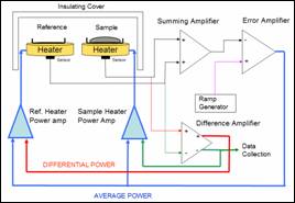
Figure 1: A “classical” DSC

Figure 1 shows a diagram of a “classical” DSC instrument. Note that this figure shows two identical heater/sensor/tray assemblies. Why is this necessary? In an ideal situation, neither the heater nor the sensor would have any mass of it's own. Neither would the holding tray. Therefore, all of the heat generated by the heater would be absorbed by the sample. The zero-mass sensor would be in intimate contact with the sample, sensing its temperature exactly, without draining off any heat of its own.

In practice this is not possible: the heater has some thermal mass, and, to a lesser extent, so do the sample tray and temperature sensor. While we can try to minimize these factors in the design of the measuring head itself, the best way to factor them out is to use two identical heater/sensor/tray assemblies. We insert our sample in the sample tray, and leave the reference tray empty and perform our measurement differentially.

Referring to Figure 1, you can see that the output signal from each sensor is added together in a summing amplifier. This signal represents the average temperature of both the Sample and Reference heater/sensor assemblies. This signal is then compared to that coming from the Ramp Generator, which is programmed to generate a ramp voltage corresponding to the sensor output voltage over the temperature range that we want to cover during our measurement run. These two signals are compared and amplified by the Error amplifier. This error signal is fed equally to both the Reference Heater Amplifier and the Sample Heater Amplifier: the net result being to bring both assemblies to the temperature called for by the ramp generator. For now just ignore the Difference amplifier and the signals that it contributes (red and green lines in the Figure 1).

Since both the Sample tray and the Reference tray are being heated equally, and only the Sample tray contains the sample material, its temperature will differ somewhat from the Reference tray. This difference will be most pronounced at the transition points, since this is where the enthalpy is the greatest. As mentioned earlier, the temperature difference at the transition points can be either positive or negative, depending upon the type of transition, and the sample material itself.

The temperature difference between the two trays is measured by the Difference amplifier. By amplifying this signal and adding it to the Average power signal going to the Reference heater amplifier, while simultaneously subtracting it from the signal going to the Sample heater amplifier, it is possible to make the temperature of both the Sample and Reference heater/trays equal to each other. Because of the Average Power signal feedback, the temperature of both heater/trays will also track the temperature signal coming from the ramp generator.

If we send the output of the Difference amplifier to a data collection system and plot it versus the ramp temperature, we will have a graph of the enthalpy. To complicate things a bit, we have to convert the Difference amplifier's output voltage into a power, since it is the heat energy we are interested in measuring, and that is proportional to the heater power applied.

Let's simplify things a bit

The method just described is used commercially and works very well. It does require two well-matched heater/sensor/tray assemblies in order to work properly, as well as two sets of control electronics. This design was developed long before the advent of computer data acquisition systems. Given a modern computerized data acquisition system, it is possible to achieve satisfactory results using only one heater/sensor/tray assembly, and associated ramped temperature controller. The idea here is to perform one run over the desired temperature range, with no sample in the tray. This Baseline information is stored in an array in the computer. Next the heater/sensor/tray is quickly cooled down to the original starting point. Then a sample is added to the tray, and another run is performed. Assuming that this is done in a timely fashion, the ambient conditions surrounding the DSC will remain constant, so the Baseline data (Reference) can be subtracted from the sample run's data, with the result being the enthalpy of the sample only.

Figure 2a

Figure 2b

Figure 2c

Figure 2a shows an actual Excel data plot obtained from my DSC with just an empty tray installed. In Figure 2b, I also plot this, as well as another dataset obtained when a small sample of Indium metal is placed in the tray. As you can see, the two traces come very close to overlaying each other, except in the melting transition region, where it is obvious that more heat had to be added to the sample to increase its temperature. Doing a subtraction of the reference data from the sample data, results in the plot shown in Figure 2c. The area under this peak is proportional to the Enthalpy of melting for Indium, and a calibration factor can be derived easily.

Figure 3 shows a block diagram of my DSC's circuit. I'll describe the heater/sensor/tray assembly in much more detail later, as it was challenging to design, but for now let's look at the overall operation of the DSC.

Figure 3- A block diagram of my DSC circuit.

I chose a Platinum Resistance Thermometer sensor (RTD) as it produces a linear output over a very wide temperature range, and produces much more signal amplitude than a thermocouple. The RTD's only disadvantage is that commonly-available commercial units are somewhat larger than the smallest thermocouples available.

Since RTDs are extremely linear, it makes sense to convert its linear resistance change into a linear voltage change, by using a constant current source. In Figure 3 you'll notice that I used a 100 ua constant-current source to feed the RTD, as well as a matched source to feed a 500 ohm precision resistor. Configuring this in a Wheatstone bridge, allows me to cancel out the 500? that this particular RTD exhibits at 0°C . The bridge voltage is amplified by an instrumentation amplifier with a voltage gain of 52. This value was chosen to convert the RTD's 0.192mv/°C signal into a 10 mv/°C signal. This is chosen because the DAC produces 1 mv per bit. This allows the DAC to be programmed for any given temperature by sending it a value equal to ten times the temperature in °C.

The two matched 100 ua constant current sources are provided by a single Burr-Brown REF200AP, which provides two very accurate and well-matched 100 ua current sources, having a very low temperature coefficient.

The sensor preamplifier's 10mv/°C output, and the DAC's output are compared and amplified in the Error Amplifier, which, like the preamp, is a Burr-Brown INA103 instrumentation amplifier. The Error Amplifier has a gain of 24, which results in an output voltage of 240mv for every °C that the sensor temperature differs from the DAC set-point temperature. The full-scale range of the ADC is +/-500 mv, corresponding to an error temperature of +/- 2°C .

The DAC is a Burr-Brown DAC7611 12 bit SPI DAC containing an internal voltage reference. Its output full-scale voltage is fixed at 4.096 volts.

Since the RTD output voltages are small, it makes sense to reduce noise as much as possible. Much of the noise present will be 60 Hz noise from the power lines. I decided to use a high-resolution Dual-Slope Integrator ADC, and chose an integration period of exactly 1/60 second. This method eliminates any 60 Hz noise from the signal after it is digitized. The ICL7135 ADC has a resolution of +/- 20000 counts and its integration period is derived from its clock frequency. The ICL7135 is extremely easy to interface with an MCU, needing only two lines and is very accurate. Furthermore, the 600 KHz clock needed by the ICL7135 can be easily provided by the ATMega8's Timer2 module. The ICL7135 is an old friend of mine, having used it for the first time 20 years ago, when Intersil first introduced it. Although Intersil is long-gone, Texas Instruments now manufactures it. It's now cheaper and more readily available than ever.

During a run, the ATMega8 MCU will output values to the DAC to form a constant temperature ramp beginning at he desired starting temperature and ending at the desired final temperature. The ramp rate is chosen by the user. The MCU will constantly monitor the Error Amplifier output voltage, digitized by the ICL7135 ADC, and will output a heater power based upon this error, in an attempt to equalize the sample temperature and the current set-point temperature. This process is repeated 15 times per second.

The power that the MCU sends out to the heater is handled by a 16-bit PWM module in the ATMega8. The PWM output switches a MOSFET which provides the heater with power from a well-regulated 16 volt supply. Since the voltage is constant, and the heater resistance is constant over temperature to within 1%, the heating power is directly proportional to the PWM's duty cycle. The heater I use is a 20 W , 5 Watt unit, which I'll describe in more detail later.

At the fastest ramp rate, the temperature ramps up 1°C every 3 seconds. Since the temperature control algorithm running in the ATMega8 does 15 updates/second, there are at least forty-five 16-bit resolution heater power readings that are added together and used as an average heating power for every 1°C increment in temperature. This accumulated power reading, for each 1°C temperature increase, is transmitted to the host PC using the ATMega8's SCI port

Conclusions

Giving students a chance to learn about enthalpy in the lab using a real DSC has been quite rewarding. There was absolutely no chance whatsoever that $60,000 would have been available to buy a commercial instrument, and even if the funds were available, such an instrument would have been too susceptible to carelessness on the part of undergraduate students, to be practical.

Although fine for demonstrating the principle of enthalpy to students in a lab, I recognize that the sensitivity of my measuring head is much less than that of commercial instruments. During the development of this project, I came up with the idea of using modern non-contact IR measurement sensors for a better version of my DSC. I am currently pursuing this project now.

[ВВЕРХ] [ГЛАВНАЯ] [ПОРТАЛ МАГИСТРОВ ДОННТУ] [ПОРТАЛ ДОННТУ]