Influence of Locomotive Tractive Effort on the Forces Between Wheel and Rail

• exact theory by Kalker (programme CONTACT)

• simplified theory by Kalker (programme FASTSIM)

• look-up tables

• simplified formulae and saturation functions.

The exact theory by Kalker (computer programme CONTACT [5]) has not been used in the simulations because of its very long calculation time. The simplified theory used in Kalker's programme FASTSIM [3] is much faster than the exact theory, but the calculation time is still relatively long for on-line computation in complicated multi-body systems. FASTSIM is used e. g. in the railway vehicle simulation tools ADAMS/Rail, MEDYNA, SIMPACK, GENSYS, VOCO. Another possibility for computer simulations consists in the use of look-up tables with saved pre-calculated values (ADAMS/Rail, VAMPIRE). Because of the limited data in the look-up table, there are differences to the exact theory as well. Large tables are more exact, but the searching in such large tables consumes calculation time. Searching for faster methods some authors found approximations based on saturation functions (e.g. Vermeulen-Johnson [12], Shen-Hedrick-Elkins [11]). The calculation time using these approximations is short, but there are significant differences to the exact theory especially in the presence of spin. Simple approximations are often used as a fast and less exact alternative to standard methods (e. g. in MEDYNA, VAMPIRE, SIMPACK). A very good compromise between the calculation time and the required accuracy allows a fast method for the computation of wheel-rail forces developed by the author [7], [8]. In spite of the simplifications used, spin is taken into consideration. Due to the short calculation time, the method can be used as a substitute for Kalker's programme FASTSIM to save computation time or instead of approximation functions to improve the accuracy. The proposed method has been used in the simulations in different programmes since 1990. The algorithm is implemented in ADAMS/Rail as an alternative parallel to FASTSIM and to the Table-book. The calculation time is faster than FASTSIM's and usually faster than the Table-book as well. The proposed algorithm provides a smoothing of the contact forces in comparison with the Table-book and there are no convergence problems during the integration. The programme was tested as user routine in programmes: SIMPACK, MEDYNA, SIMFA and various user's own programmes with very good experience.

The proposed method assumes an ellipsoidal contact area with half-axes a, b and normal stress distribution according to Hertz. The maximum value of tangential stress r at any arbitrary point is

where f - coefficient of friction,

e - normal stress.

The coefficient of friction / is assumed constant in the whole contact area. The solution described in [7], [8] obtains the resultant tangential force (without spin) as

where Q - wheel load

a,b- half-axes of the contact ellipse

s - creep

where Q - wheel load

where sx, sy - creep in longitudinal (x) and lateral (y) directions

wx, wy - creep (slip) velocity in longitudinal (x) and lateral (y) directions

V - vehicle speed.

Using the Kalker's linear theory to express the coefficient C, the equation (3) has then the form (in the case of only longitudinal creep)

where c11 - Kalker's coefficient for longitudinal direction [2].
The calculation of tangential forces for general case with combination of longitudinal and lateral creep and spin allows the computer code published in [8]. The proposed method was verified by making a comparison between curving behaviour calculations using for the computation of wheel-rail forces the programme FASTSIM and the proposed method, and by comparison with measurements. A model of the four axle SBB 460 locomotive of the Swiss Federal Railways was built by means of the simulation tool ADAMS/Rail. The locomotive design combines very good curving performance with high maximal speed due to the coupling of wheelsets, realised by a mechanism with a torsional shaft assembled to the bogie frame. The model used in simulations consists of 51 rigid bodies and contains 266 degrees of freedom. Fig. 1. Measured lateral wheel-rail forces in a curve with 300 m radius compared with the simulations using the method developed by the author [8] and using FASTSIM. The results using both calculation methods mentioned are similar, see Fig. 1. However, there is a significant difference in the calculation time. The results computed using the proposed method show good agreement with the measurements. Especially in the case of the leading wheelsets, they are nearer to the actually measured values than the results obtained in the simulations using FASTSIM.

3. DIFFERENCES BETWEEN THE VEHICLE DYNAMICS AND AXLE DRIVE DYNAMICS

Depending on the aim of the tests, different measured creep-force functions can be found in the literature [6], Because of the variety of measurements different models are used for the same physical phenomenon - forces between wheel and rail - in the vehicle dynamics and axle drive dynamics (Fig. 2). How is this possible? The reason for this are different fields of parameters and different areas of investigations. In the vehicle dynamics small creep values are of main importance. Tangential forces in longitudinal as well as in lateral directions influence the vehicle behaviour, therefore longitudinal and lateral creep as well as spin should be taken into account Based on the theory of rolling contact, the creep forces depend on the creep as non-dimensional value. The friction coefficient is assumed to be constant. The difference between dry and wet conditions is usually expressed only with the value of friction coefficient and not with a change of the creep-force function gradient.

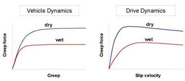
Fig. 1. Differences between the typical creep-force functions used in the vehicle dynamics and in axle drive dynamics.
In the drive dynamics large values of longitudinal creep influence its behaviour. In the simulated systems usually only the longitudinal direction is taken into account Based on the experiments, the creep forces are usually assumed as dependent on the slip velocity between wheel and rail. There is a maximum of creep-force function, so called adhesion optimum, and a decreasing section behind this maximum. The gradient and the form of creep-force functions for wet, dry or other conditions are different.

4. MODEL OF WHEEL-RAIL FORCES USEFUL FOR SIMULATION OF VEHICLE DYNAMICS AND AXLE DRIVE DYNAMICS INTERACTION

For the complex simulation of dynamic behaviour of locomotive or traction vehicle in connection with drive dynamics and traction control, high longitudinal creep and decreasing section of creep-force function behind the adhesion limit has to be taken into account. The different wheel-rail models described above have to be made into one model, which is suitable for both vehicle dynamics and drive dynamics simulations. A creep-force law with a marked adhesion optimum can be modelled using the friction coefficient decreasing with increasing slip (creep) velocity between wheel and rail. The dependence of friction on the slip velocity was observed by various authors and is described e. g. in [6], [9]. The variable friction coefficient can be expressed by the following equation

where fo- maximum friction coefficient

w- magnitude of the slip (creep) velocity vector [m/s]

B - coefficient of exponential friction decrease [s/m]

A - ratio of limit friction coefficient at infinity slip velocity to maximum friction coefficient fo, A= / fo.

From the point of view of tractive effort and traction dynamics the creep law for bad adhesion conditions is of main importance: wet rail and surface pollution e. g. oil, dirt, moisture. Even for dry conditions the gradient of creep-force functions is usually lower than the theoretical value. The reason of this is the layer of moisture, which can be taken into consideration in the "stiffness coefficient" of surface soil [4]. In the vehicle dynamics, this real conditions are taken into account simply with a reduction of Kalker's creep coefficients [2]. This method is used for the linear creep force law but can be used generally as well.

library