
Content
- Introduction
- 1. Relevance of the topic
- 2. The purpose and objectives of the study
- 3. Development of a method of determining the constants of empirical formulas for calculating the flow stress of the metal
- 3.1 Ensuring high accuracy of definition of G, depending on e, U, T on the basis of the curves
- 3.2 Scientific and informed choice of the most rational points in the range of the factorse, U, T to determine the appropriate values of G
- 4. The results of the Conclusions.
- Conclusions
- List of sources
Introduction
At the present time in the technical literature, there are extensive experimental data on the flow stress of the metal from the G strain e, strain rate U and temperature T, presented in the form of hardening curves. In several cases, including the development of computer programs is necessary to develop empirical formulas, which are necessary for the calculation of the flow stress of metals G.
1. Relevance of the topic
An urgent task is to obtain empirical formulas for calculating the flow stress of metal for construction, tool and stainless steels based on the available experimental plastometric information.
2. The purpose and objectives of the study
The aim is to develop a method for determining the constants of empirical formulas for calculating the flow stress of metal for construction, tool and stainless steels based on the available experimental data plastometric.
After selecting the type of empirical formula is required to determine the constants occurring in it, based on available experimental information on the work-hardening curves. In this case there are two urgent tasks:
- To ensure high accuracy of definition of G, depending on e, U, T on the basis of hardening curves;
- Implement evidence-based selection of the most rational points in the range of the factors e, U, T to determine the appropriate value G.
3. Development of a method of determining the constants of empirical formulas for calculating the flow stress of the metal
3.1 Ensuring high accuracy of definition of G, depending on e, U, T on the basis of work-hardening curves
To solve the first problem it is advisable to develop a computer program for determining the values of G by spline - interpolation of experimental data [2], [3].
Since the experimental information can be presented in different forms, has developed several windows presentation of experimental data (Fig. 1, 3).

Figure 1 - The program window for a set of graphs at different strain rates and the fixed temperature.

Figure 2 - The program window for a set of graphs with ke, ku, kT.
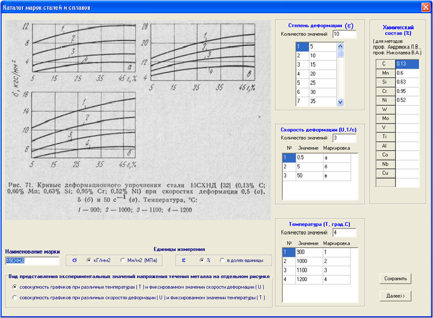
Figure 3 - The program window for a set of graphs at different temperatures and a fixed value of strain rate.
Determination of the quantities G, depending on the arbitrary values of e, U, T invited to perform as follows. In the first stage of the window a computer program recorded the scanned curves of hardening. The original data set (Fig. 1, 3).
Once given all the necessary background information necessary to determine the coordinates of nodal points on the axes in units of raster images.
In the program window (Figure 4) for all nodal points of the coordinate axes are mapped to values of G and e in units as specified on the coordinate axes, as well as in units of raster images, which are defined by software. Running a graphical visualization of the constructed lines, which is necessary to ensure the most accurate matching network built in a different color from the original grid. In the program window (Figure 4) for all nodal points of the coordinate axes are mapped to values of G and e in units as specified on the coordinate axes, as well as in units of raster images, which are defined by software. Running a graphical visualization of the constructed lines, which is necessary to provide the most accurate matching network built in a different color from the original grid.

Figure 4 - The window construction of the grid
Based on this information for any point on the graph, we can determine the abscissa and ordinate in raster units, and then calculate them in the units specified on the coordinate axes. The program calculates the values of the flow stress of the metal G (e, U, T) and writes them to the table.
Performed stepwise change in the value of factors e, U, T, values obtained flow stress of the metal stored in a table. You must completely fill in the table of experimental values.
Handled all the curves of hardening in the whole range of factors, e, U, T.
Next, spline interpolation is performed to the information received and the construction of spline - the curves in the window (Figure 5). If the initial course of the hardening curve is rather complicated, for example, there are excesses and spline - curve is not accurately placed on the original curve, it is possible to increase the number of points and achieve a complete coincidence of the interpolation curve and the original one.

Figure 5 - Window removal of experimental information and control the construction of spline - curves.
In Table. 1 shows an experimental digital data from the curves of hardening in the whole range of factors, e, U, T.
Table 1 - Experimental digital information from the curves of hardening
| e | 5 | 10 | 15 | 20 | 25 | 30 | 35 | 40 | 45 | 50 |
| T=900, U=0,5 | 7.933 | 8.828 | 9.586 | 10.207 | 10.793 | 11.207 | 11.517 | 11.655 | 11.724 | 11.690 |
| T=900,U=5 | 10.400 | 11.511 | 12.489 | 13.333 | 14.087 | 14.783 | 15.391 | 15.826 | 16.261 | 16.609 |
| T=900,U=50 | 13.333 | 15.373 | 17.098 | 18.588 | 19.843 | 21.067 | 21.981 | 22.743 | 23.352 | 23.810 |
| T=1000,U=0,5 | 5.546 | 6.319 | 6.891 | 7.395 | 7.798 | 8.103 | 8.345 | 8.483 | 8.586 | 8.552 |
| T=1000,U=5 | 7.565 | 8.609 | 9.435 | 10.178 | 10.800 | 11.378 | 11.867 | 12.267 | 12.489 | 12.667 |
| T=1000,U=50 | 10.231 | 12.000 | 13.490 | 14.824 | 16.000 | 17.020 | 17.882 | 18.431 | 18.980 | 19.216 |
| T=1100,U=0,5 | 3.322 | 3.966 | 4.471 | 4.908 | 5.210 | 5.445 | 5.613 | 5.748 | 5.782 | 5.782 |
| T=1100,U=5 | 5.455 | 6.304 | 7.043 | 7.609 | 8.130 | 8.565 | 8.913 | 9.217 | 9.391 | 9.478 |
| T=1100,U=50 | 8.154 | 9.615 | 10.769 | 11.769 | 12.549 | 13.255 | 13.725 | 14.039 | 14.275 | 14.353 |
| T=1200,U=0,5 | 2.034 | 2.542 | 2.983 | 3.322 | 3.593 | 3.831 | 3.966 | 4.034 | 4.000 | 3.932 |
| T=1200,U=5 | 4.045 | 4.591 | 5.136 | 5.591 | 5.955 | 6.217 | 6.391 | 6.522 | 6.565 | 6.478 |
| T=1200,U=50 | 6.000 | 7.154 | 8.077 | 8.846 | 9.308 | 9.692 | 10.000 | 10.154 | 10.154 | 9.923 |
Created window (Figure 6) allows to determine the values of the flow stress of the metal at fixed values of e, U, T. These values are calculated as follows.
In the first phase, the spline interpolation of the initial information on the basis of third-degree polynomials.
In the next stage when e = e * is calculated first array G for given values of the information in the original factors of U and T. The calculation results are shown in the table at the top of the window.
After performing a spline interpolation of the data given by the value of an additional U = U * is calculated, and the second array G as defined in the original data values of the factor T. The calculation results are displayed in another table, below.
In the final step is the interpolation of the data and calculates the required value of G at t = T *.

Figure - 6 program window spline interpolation curves of hardening
3.2 Scientific and informed choice of the most rational points in the range of the factors e, U, T to determine the appropriate values of G
To solve the second problem, it is proposed to apply the method of calculation of the planned experiment [5]. Created window (see Figure 7) where a table located in the upper part, passed the limits of variation factors e, U, T. In the same window formed a table of code values and natural factors. In accordance with the theory of planned experiment, the plan is the matrix for the 3 factors e, U, T always contains 15 lines to determine the values of G. The planned experiment covers the entire range of the factors e, U, T, and determines the most rational point for determining the values of G on the basis of experimental data. And it is a science-based theory of planned experiment a minimum of experiments.
To become 15СХНД shows the values of the flow stress of the metal seksp obtained by spline interpolation curves of hardening. Under the proposed method are found in the constant in the formula of Professor. V.I. Zyuzin [1], and on this basis calculated the values of Gp. The values of the constants are presented in the right pane, calculated by the method of least squares. Also found an average relative deviation of calculated values of gp, from the corresponding experimental values Geksp equal to 2.5%.

Figure 7 - Windows program for calculation of the constants in the formula V.I. Zyuzin
4. The results of the Conclusions
By using the proposed method of determining the constants of empirical formulas for calculating the flow stress of the metal and the developed computer program was carried out calculations of the constants in the formula V.I. Zyuzin [1] for 36 grades of steel. The average relative error of approximation of experimental data for all grades according to the formula of Professor. Zyuzin [1] was 4.7%. The constants are presented in Table 2.
Table 2 - Constants in the formula of Professor. V.I. Zyuzin
| Steel | A , МПа | n1 | n2 | n3 | Error, % |
| У8,[6],стр.156, рис.107 | 1821 | 0,233 | 0,196 | 0,00294 | 2,2 |
| У12А,[6],стр.159, рис.111 | 1447,9 | 0,24025 | 0,15444 | 0,0024765 | 8,3 |
| У12А,[7],стр.83, рис.33 | 5951,3 | 0,18979 | -0,15356 | 0,003304 | 10 |
| X17H2,[6],стр.200, рис.164 | 6453,8 | 0,25152 | 0,06584 | 0,003656 | 3,2 |
| Х12,[6],стр.185, рис.139 | 2882,3 | 0,22104 | 0,0765 | 0,0025331 | 3,1 |
| ХВГ,[6],стр.137, рис.79 | 3472,5 | 0,25561 | 0,13761 | 0,0029445 | 4,2 |
| ХВГ,[7],стр.85, рис.35 | 4279,3 | 0,28837 | 0,13308 | 0,0030085 | 5,1 |
| Р18,[6],стр.168, рис128 | 4834,5 | 0,1629 | 0,0675 | 0,0030983 | 5,1 |
| Р18,[6],стр.169, рис.130 | 3118,4 | 0,20879 | 0,12924 | 0,0028369 | 2,1 |
| Cт3,[6],стр.101, рис.22 | 1846,1 | 0,23057 | 0,1521 | 0,0028402 | 2,3 |
| Сталь 45,[6],стр.105, рис.28 | 1935,6 | 0,27336 | 0,17505 | 0,0028004 | 16,4 |
| Сталь 45,[6],стр.105, рис.29 | 1733,1 | 0,23969 | 0,14375 | 0,0027614 | 3,1 |
| Сталь 55,[6],стр.108, рис.37 | 2250,6 | 0,23481 | 0,15406 | 0,0029966 | 2 |
| 12ХН3А,[6],стр.146, рис.97 | 1955,2 | 0,24089 | 0,13244 | 0,0027751 | 2,6 |
| 14ГН, [6],стр.119, рис.49 | 2055,7 | 0,24508 | 0,15734 | 0,0028744 | 2,5 |
| 15СХНД,[6],стр.133, рис.71 | 1871,5 | 0,25049 | 0,16055 | 0,002806 | 2,5 |
| 18ХНВА,[6],стр.137, рис.80 | 3126,2 | 0,29523 | 0,10937 | 0,0027974 | 3,9 |
| 18ХНВА,[7],стр.87, рис.37 | 12113,6 | 0,25072 | -0,11248 | 0,003671 | 11,5 |
| 40X,[6],стр.122, рис.52 | 2183,9 | 0,24376 | 0,14499 | 0,0029576 | 3,5 |
| 60C2,[6],стр.161, рис.114 | 2174,9 | 0,20983 | 0,15854 | 0,0028432 | 2,7 |
| 60С2,[6],стр.161, рис.113 | 3546,3 | 0,21555 | 0,08984 | 0,0032892 | 3,8 |
| 60С2[7],стр.84, рис.34 | 4148,2 | 0,247 | 0,07593 | 0,0032819 | 3,5 |
| ШХ15,[6],стр.163, рис.118 | 1855,2 | 0,21926 | 0,15687 | 0,0028206 | 2,7 |
| 2Х18Н9,[7],стр.89, рис.39 | 2365,2 | 0,2643 | 0,11194 | 0,0022885 | 4,1 |
| 4Х13,[7],стр.86, рис. 36 | 2146,6 | 0,25424 | 0,07646 | 0,001976 | 4,3 |
| 10Х17Н13М2Т,[6],стр.219,рис.192 | 7018,7 | 0,27233 | 0,03964 | 0,0030591 | 6 |
| 10Х17Н13М2Т,[6],стр.221,рис.195 | 2685 | 0,23885 | 0,14783 | 0,0027323 | 1,9 |
| 12X13,[6],стр.186, рис.141 | 11889,9 | 0,29699 | 0,08867 | 0,0041241 | 6,6 |
| 12X13,[6],стр.187, рис.142 | 3491,1 | 0,25718 | 0,16121 | 0,0031423 | 4,6 |
| 12Х18Н9Т,[6],стр.207, рис.177 | 2394,2 | 0,25237 | 0,07633 | 0,0025765 | 2,8 |
| 12Х18Н9Т,[6],стр.211, рис.181 | 4234.0 | 0,25968 | 0,07041 | 0,0026974 | 4,7 |
| 20Х23H18,[6],стр.223, рис.199 | 9230,2 | 0,26303 | 0,09778 | 0,0036406 | 8 |
| 40Х13,[6],стр.190, рис.149 | 5602,1 | 0,24724 | 0,06111 | 0,0035183 | 3,2 |
| 40Х13,[6],стр.191, рис.150 | 3394,2 | 0,20741 | 0,10326 | 0,0028074 | 4,5 |
| Х18Н9Т,[7],стр.88, рис.38 | 4017,1 | 0,21782 | 0,1013 | 0,0029308 | 5,2 |
| Х18Н25С2,[6],стр.225, рис.202 | 6969,8 | 0,17122 | 0,05129 | 0,0032477 | 6,2 |
The calculation of the constants included in the second degree polynomial [4]. The average relative error of approximation of experimental data for all grades of 5.2% formula. The constants are presented in Table 3.
Table 3 - The constants included in the second degree polynomial
| Stell | a0 | a1 | a2 | a3 | a4 | a5 | a6 | a7 | a8 | a9 | a10 | Error, % |
| У8,[6],стр.156,рис.107 | 971,79 | -117,73 | -0,019373 | 0,000681 | 380,1 | 3,523 | -1,6063 | 6,732 | -0,23269 | -0,0016206 | -0,0047786 | 4,7 |
| У12А,[6],стр.159,рис.111 | 1013,38 | -179,65 | -0,002575 | 0,000684 | 299,47 | 1,204 | -1,6464 | 5,664 | -0,10009 | -0,000287 | -0,0047221 | 6,4 |
| У12А,[7],стр.83,рис.33 | 361,11 | -1934,6 | 0,005728 | -0,000002 | 867,6 | -1,794 | -0,281 | -0,152 | -0,03788 | 0,0005897 | -0,0006526 | 15,2 |
| X17H2,[6],стр.200,рис.164 | 911,22 | -530,42 | -0,012062 | 0,000517 | 781,26 | 2,203 | -1,3648 | 3,733 | -0,4002 | -0,0011977 | -0,0025991 | 3,2 |
| Х12,[6],стр.185,рис.139 | 2361,99 | -68,81 | -0,004431 | 0,001669 | 667,65 | 0,363 | -3,9161 | 1,992 | -0,41832 | 0,0005091 | -0,0014959 | 5,4 |
| ХВГ,[6],стр.137,рис.79 | 2957,95 | -200,75 | -0,006177 | 0,002298 | 1053,76 | 1,68 | -5,1827 | 0,049 | -0,73653 | -0,0003474 | 0,0005761 | 9,8 |
| ХВГ,[7],стр.85,рис.35 | 3227,27 | -241,81 | -0,005607 | 0,002511 | 1264,07 | 1,39 | -5,6576 | 1,562 | -0,90406 | -0,0002568 | -0,0001453 | 8,8 |
| Р18,[6],стр.168,рис128 | 1536,33 | -390,54 | -0,062706 | 0,000919 | 431,37 | 13,648 | -2,3422 | 18,893 | -0,1389 | -0,008926 | -0,0095226 | 0,8 |
| Р18,[6],стр.169,рис.130 | 1206,42 | -195,12 | -0,029542 | 0,000717 | 695,37 | 3,677 | -1,8295 | 3,776 | -0,42954 | -0,0010825 | -0,0025322 | 4,4 |
| Cт3,[6],стр.101,рис.22 | 806,16 | -135,6 | -0,016365 | 0,000508 | 397,36 | 2,382 | -1,2601 | 4,098 | -0,23401 | -0,0008692 | -0,0026443 | 4,8 |
| Сталь 45,[6],стр.105,рис.28 | 783,58 | -437,71 | -0,001826 | 0,000479 | 757,46 | 1,718 | -1,2327 | -0,43 | -0,39957 | -0,0007308 | 0,0010493 | 8,8 |
| Сталь 45,[6],стр.105,рис.29 | 758,1 | -246,46 | -0,012169 | 0,000474 | 482,88 | 1,559 | -1,1833 | 4,413 | -0,26031 | -0,0002575 | -0,003208 | 4,4 |
| Сталь 55,[6],стр.108,рис.37 | 920,66 | -132,88 | -0,017421 | 0,000594 | 396,35 | 2,677 | -1,4614 | 5,093 | -0,22086 | -0,0009506 | -0,0039443 | 4,5 |
| 12ХН3А,[6],стр.146,рис.97 | 623,28 | -368,64 | -0,014707 | 0,000359 | 549,81 | 3,176 | -0,9344 | 3,492 | -0,2631 | -0,001618 | -0,0024437 | 4,3 |
| 14ГН, [6],стр.119,рис.49 | 844,26 | -117 | -0,016021 | 0,000527 | 415,08 | 2,279 | -1,3167 | 5,675 | -0,24186 | -0,0006316 | -0,0043089 | 4,4 |
| 15СХНД,[6],стр.133,рис.71 | 773,95 | -129,56 | -0,015768 | 0,000473 | 403,76 | 1,869 | -1,1936 | 6,883 | -0,22978 | -0,0003161 | -0,0052415 | 4,9 |
| 18ХНВА,[6],стр.137,рис.80 | 2026,1 | -427,65 | -0,004213 | 0,001479 | 615,59 | 1,419 | -3,4401 | 2,681 | -0,23134 | -0,0004947 | -0,0017936 | 8,7 |
| 18ХНВА,[7],стр.87,рис.37 | 1063,21 | -1728,48 | 0,003461 | 0,000568 | 1230,83 | -1,526 | -1,5319 | 3,135 | -0,39259 | 0,0005711 | -0,003358 | 8,9 |
| 40X,[6],стр.122,рис.52 | 647,31 | -130,87 | -0,018208 | 0,00036 | 316,75 | 3,606 | -0,951 | 4,513 | -0,15923 | -0,0020224 | -0,002841 | 5,1 |
| 60C2,[6],стр.161,рис.114 | 869,3 | -125,3 | -0,018206 | 0,000502 | 395,81 | 2,751 | -1,301 | 6,733 | -0,22807 | -0,0008681 | -0,004979 | 4,1 |
| 60С2,[6],стр.161,рис.113 | 1766,6 | -153,81 | -0,002393 | 0,001276 | 371,41 | 0,979 | -2,977 | 1,123 | -0,19894 | -0,0003961 | -0,0006674 | 4,8 |
| 60С2[7],стр.84,рис.34 | 1572,59 | -298,19 | -0,001933 | 0,001123 | 575,59 | 1,033 | -2,6333 | 1,637 | -0,30368 | -0,0005012 | -0,0012188 | 3,7 |
| ШХ15,[6],стр.163,рис.118 | 792,46 | -162,11 | -0,012802 | 0,000487 | 316,46 | 2,319 | -1,2236 | 9,614 | -0,14116 | -0,0008038 | -0,007971 | 4,2 |
| 2Х18Н9,[7],стр.89,рис.39 | 2521,91 | -369,18 | -0,005893 | 0,001792 | 591,16 | 1,294 | -4,2186 | 0,179 | -0,15333 | 0,0000523 | 0,0001038 | 8,7 |
| 4Х13,[7],стр.86, рис. 36 | 2755,96 | -749,54 | -0,003478 | 0,002081 | 1061,77 | 0,094 | -4,7245 | 6,823 | -0,48056 | 0,0006962 | -0,0054642 | 4,1 |
| 10Х17Н13М2Т,[6],стр.219,рис.192 | 735,59 | -506,13 | -0,002576 | 0,00015 | 1236,58 | 1,735 | -0,7566 | -1,965 | -0,69106 | -0,0010672 | 0,0022645 | 3,3 |
| 10Х17Н13М2Т,[6],стр.221,рис.195 | 1257,16 | -184,28 | -0,02875 | 0,000791 | 605,52 | 3,023 | -1,9635 | 8,573 | -0,35592 | -0,0005825 | -0,0061543 | 4,4 |
| 12X13,[6],стр.186,рис.141 | 1727,97 | -515,86 | -0,066632 | 0,001244 | 627,32 | 24,993 | -2,9165 | 21,584 | -0,27793 | -0,020722 | -0,0080364 | 2 |
| 12X13,[6],стр.187,рис.142 | 1138,39 | -163,12 | -0,025339 | 0,00067 | 483,53 | 1,799 | -1,7426 | 9,773 | -0,2348 | 0,0006653 | -0,0086492 | 4,3 |
| 12Х18Н9Т,[6],стр.207,рис.177 | 1003,69 | -615,22 | -0,012176 | 0,000658 | 884,41 | 3,44 | -1,6001 | -3,65 | -0,42473 | -0,0020676 | 0,0036643 | 3,3 |
| 12Х18Н9Т,[6],стр.211,рис.181 | 1889,19 | -532,68 | -0,003032 | 0,00121 | 921,48 | 1,179 | -2,9902 | 1,919 | -0,40154 | -0,0003034 | -0,0013529 | 4,6 |
| 20Х23H18,[6],стр.223,рис.199 | 2986,63 | -426,26 | -0,156398 | 0,002202 | 725,38 | -7,246 | -5,1001 | 60,347 | -0,38106 | 0,0102688 | -0,0389154 | 2,3 |
| 40Х13,[6],стр.190,рис.149 | 857,42 | -544,18 | -0,009708 | 0,000482 | 812,35 | 2,432 | -1,2781 | 0,584 | -0,41586 | -0,0014521 | -0,0001192 | 3,7 |
| 40Х13,[6],стр.191,рис.150 | 2052,57 | -393,28 | -0,003381 | 0,001418 | 575,52 | 2,26 | -3,3689 | 0,74 | -0,25155 | -0,0012538 | 0,0000705 | 5,7 |
| Х18Н9Т,[7],стр.88,рис.38 | 1919,82 | -408,98 | -0,003145 | 0,001285 | 616,15 | 2,574 | -3,1008 | -0,57 | -0,28577 | -0,0015789 | 0,0014448 | 5,2 |
| Х18Н25С2,[6],стр.225,рис.202 | 1810,36 | -639,99 | 0,100446 | 0,001078 | 1257,14 | 2,269 | -2,7517 | -70,439 | -0,80171 | 0,0000092 | 0,0761921 | 0,9 |
The analysis of the accuracy of "self-contained" methods of prof. Nikolayev [8] and the method of prof. Andreyuk [9].
The planned experiment involving 15 settlements quantities G, covers the entire range of the factors e, U, T, and determines the most rational point for the comparison of experimental and calculated values of G [5].
Calculations carried out for 27 grades of steel. Found that the average relative error of the method of Nikolaev VA. [8] was 14.5% (the maximum relative error (for steel R18, see Chart 4) is equal to 32.3%). The average relative error of the method Andreyuk L. et al [9] was 21.2% (the maximum relative error (for steel R18, see Chart 4) is equal to 67%). In carrying out the calculations for the considered steels was determined by a number of constants appearing in the formulas of methods, which are presented in the table 4.
Table 4 - Constants included in the method of Nikolaev V.A. and the method of L.V. Andreyuk
| Steel [6] | The limits of change factors | Method of Nikolaev V.A | Method of L.V. Andreyuk | e | U, с-1 | G0, МПа | Error, % | N | A | B | C | Error, % |
| Cт3, стр.101, рис.22 | 0,05-0,5 | 0,5-50 | 88,353 | 6,56 | 74,777 | 0,134 | 0,186 | -2,957 | 4,97 |
| Сталь 45, стр.105, рис.28 | 0,05-0,5 | 0,05-150 | 91,313 | 18,2 | 75,195 | 0,148 | 0,186 | -3,369 | 18,39 |
| Сталь 45, стр.105, рис.29 | 0,05-0,4 | 0,5-50 | 88,353 | 5,35 | 74,691 | 0,144 | 0,193 | -3,003 | 7,83 |
| Сталь 55, стр.108, рис.37 | 0,05-0,5 | 0,5-50 | 90,46 | 7,56 | 75,783 | 0,143 | 0,199 | -2,977 | 4,34 |
| 12ХН3А, стр.146, рис.97 | 0,05-0,4 | 0,5-50 | 104,924 | 12,19 | 100,273 | 0,116 | 0,185 | -2,806 | 24,95 |
| 14ГН, стр.119, рис.49 | 0,05-0,5 | 0,5-50 | 98,928 | 6,23 | 90,933 | 0,124 | 0,19 | -3,065 | 13,19 |
| 15СХНД, стр.133, рис.71 | 0,05-0,5 | 0,5-50 | 98,274 | 7,54 | 86,713 | 0,117 | 0,185 | -2,943 | 10,04 |
| 18ХНВА, стр.137, рис.80 | 0,05-0,45 | 0,05-150 | 111,419 | 14,52 | 100,72 | 0,119 | 0,206 | -2,954 | 8,9 |
| 40X, стр.122, рис.52 | 0,05-0,5 | 0,5-50 | 97,992 | 9,86 | 88,577 | 0,136 | 0,208 | -3,125 | 21,05 |
| 60C2, стр.161, рис.114 | 0,05-0,5 | 0,5-50 | 101,825 | 12 | 76,032 | 0,149 | 0,207 | -3,166 | 12,54 |
| 60С2, стр.161, рис.113 | 0,05-0,5 | 0,05-150 | 100,711 | 9,57 | 72,959 | 0,154 | 0,203 | -3,211 | 12,45 |
| ШХ15, стр.163, рис.118 | 0,05-0,5 | 0,5-50 | 100,05 | 7,78 | 94,082 | 0,152 | 0,202 | -3,173 | 26,87 |
| У8, стр.156, рис.107 | 0,05-0,5 | 0,5-50 | 91,769 | 10,05 | 77,8 | 0,15 | 0,198 | -2,992 | 12,47 |
| У12А, стр.159, рис.111 | 0,05-0,4 | 0,05-150 | 91,542 | 11,49 | 80,509 | 0,158 | 0,173 | -2,987 | 10,94 |
| X17H2, стр.200, рис.164 | 0,05-0,4 | 0,5-50 | 112,357 | 12,52 | 123,742 | 0,116 | 0,118 | -3,597 | 38,14 |
| Х12, стр.185, рис.139 | 0,05-0,4 | 0,05-150 | 111,227 | 30,03 | 140,38 | 0,148 | 0,144 | -3,711 | 21,88 |
| ХВГ, стр.137, рис.79 | 0,05-0,5 | 0,05-150 | 104,619 | 28,97 | 82,604 | 0,157 | 0,222 | -3,432 | 22,17 |
| Р18, стр.168, рис128 | 0,05-0,5 | 0,05-7,5 | 114,492 | 32,32 | 195,135 | 0,151 | 0,117 | -3,985 | 29,89 |
| Р18, стр.169, рис.130 | 0,05-0,5 | 0,5-50 | 115,059 | 23,7 | 210,405 | 0,122 | 0,076 | -2,409 | 66,96 |
| 10Х17Н13М2Т, стр.219,рис.192 | 0,05-0,5 | 0,05-150 | 158,669 | 13,91 | 179,823 | 0,103 | 0,107 | -3,14 | 17,7 |
| 10Х17Н13М2Т, стр.221,рис.195 | 0,05-0,5 | 0,5-50 | 139,018 | 7,96 | 168,776 | 0,097 | 0,09 | -2,716 | 28,5 |
| 12X13, стр.186, рис.141 | 0,05-0,4 | 0,05-7,5 | 111,212 | 17,79 | 126,52 | 0,116 | 0,161 | -3,681 | 22,32 |
| 12X13, стр.187, рис.142 | 0,05-0,5 | 0,5-50 | 111,389 | 10,54 | 126,11 | 0,11 | 0,162 | -3,657 | 15,74 |
| 12Х18Н9Т, стр.207, рис.177 | 0,05-0,4 | 0,5-50 | 123,604 | 3,69 | 179,336 | 0,078 | 0,142 | -3,226 | 55,16 |
| 12Х18Н9Т, стр.211, рис.181 | 0,05-0,5 | 0,05-150 | 127,422 | 30,01 | 185,08 | 0,066 | 0,121 | -3,344 | 11,56 |
| 40Х13, стр.190, рис.149 | 0,05-0,4 | 0,5-50 | 111,214 | 11,54 | 124,682 | 0,127 | 0,178 | -3,713 | 44,75 |
| 40Х13, стр.191, рис.150 | 0,05-0,4 | 0,05-150 | 111,253 | 29,53 | 126,592 | 0,127 | 0,18 | -3,72 | 9,39 |
Conclusions
The solution of the problems indicated above provides a method for determining the constants of empirical formulas for calculating the flow stress of metals G.
Developing a new method based on the planned experiment and computer program allowed by the experimental information on plastometric hardening curves to determine the constants appearing in the formula for calculating the flow stress of the metal, depending on e, U, T. Received more than 120 new formulas for calculating the flow stress of metal construction, tool and stainless steels.
List of sources
- Целиков А.И. Теория прокатки: Справочник / А.И. Целиков, А.Д. Томленов, В.И. Зюзин, А.В. Третьяков, Г.С. Никитин. - М.: Металлургия, 1982. - 335с.
- Яковченко А.В. Определение напряжения течения металла с учетом истории процесса нагружения на основе уравнения А.Надаи/ А.В.Яковчеко, Н.И.Ивлева, А.А.Пугач// Наукові праці ДонНТУ. Металургія, 2011.-Вип.12(177). - С.181 - 193.
- Яковченко А.В. Анализ точности известных методов расчета напряжения течения металла в зависимости от химического состава стали / А.В. Яковченко, А.А. Пугач, Н.И. Ивлева // Вісник Приазовського державного технічного університету. Сер.: Технічні науки: Зб. наук. праць. – Маріуполь: ДВНЗ «Приазов. держ. техн. ун-т», 2011. - Вип.2(23). - С. 69 - 80.
- Данилов А.В. Анализ и усовершенствование методов расчета напряжения течения металла в процессах горячей пластической деформации. Металлургия и обработка металлов (выпуск 12) / Материалы научно-исследовательских работ студентов и молодых ученых физико-металлургического факультета ДонНТУ. – Донецк: ДонНТУ, 2009. – С. 42,43.
- Винарский, М.С. Планирование эксперимента в технологических исследованиях : учеб. пособие / М.С. Винарский, М.В Лурье. – К.: Техника, 1975. – 168 с.
- Полухин П.И. Сопротивление пластической деформации металлов и сплавов: Справочник / П.И. Полухин, Г.Я. Гун, А.М. Галкин. – М.: Металлургия, 1983. - 352с.
- Примение теории ползучести при обработке металлов давлением. Поздеев А.А., Тарновский В.И., Еремеев В.И., Баакашвили В.С. Изд-во «Металлургия», 1973, 192с.
- Николаев В.А. Теория прокатки: Монография. - Запорожье: Издательство Запорожской государственной инженерной академии, 2007. - 228с.
- Андреюк Л.В. Аналитическая зависи¬мость сопротивления деформации сталей и сплавов от их химического состава / Л.В. Андреюк, Г.Г. Тюленев, Б.С. Прицкер // Сталь. – 1972. – № 6. – C. 522, 523.