Masters Portal DonNTU

Oleg Suponin

Introduction

Technological advances have made ​​a significant step forward, and today there are so many projects, the main task is to track moving objects in space, performing various operations and control over them. In this regard, all such facilities must calculate and predict the trajectory and characteristics of their movement.

1 Relevance

Predict the behavior of a moving object is currently a topical issue, which is that it is necessary to know in advance the possible ways of object behavior depending on external factors and criteria. Need to address the time constraints associated with the calculation and determination of the location of the object.

2 Trajectory generation algorithm

Calculating the path by using different algorithms, the main ones are: the algorithm Floyd-Uorshella and Dijkstra.

2.1 Floyd–Uorshell's algorithm

This algorithm is used to find the shortest paths between all the vertices of a directed weighted graph. Developed in 1962 by Robert Floyd and Stephen Uorshellom. A more rigorous formulation of the problem is the following: [4]
a directed graph G = (V, E) with each arc v -> w of the graph compared the cost of a non-negative C [v, w]. The general problem of finding the shortest path is to find for each ordered pair of vertices v, w) of any path from vertex v in w, whose length is minimal among all possible paths from v to w.

The formal description

There are sequentially numbered from 1 to n vertices of the graph. Floyd's algorithm uses a matrix A of size n * n, which computes the length of the shortest paths. Initially, A [i, j] = C [i, j] for all i! = J. If the arc i - »j absent, C [i, j] = infinity. Each diagonal element of A is 0.

On the matrix A the n iterations. After the k-th iteration, A [i, j] contains the value shortest path from vertex i to vertex v, which do not pass through the top with a number greater k. In other words, the path between the end nodes i and may be only the peaks that are less than or equal to k. At the k-th iteration for the calculation of the matrix A, the following formul:
A_k[i,j]=min(A_k-1[i,j], A_k-1[i,k]+A_k-1[k,j])
The subscript k denotes the value of A after the k-th iteration, but it does not mean that there are n different matrices, the index used for brevity. To calculate the Ak [i, j] compares the value Ak-i [i, j] (ie the cost of the path from node i to node j without the participation of the top k or other vertex with a higher number) with an Ak-1 [ i, k] + Ak-1 [k, j] (the cost of the path from vertex i to vertex k plus the cost of the path from the top to the top k j). If the path through the vertex k less than Ak-1 [i, j], then the value Ak [i, j] is changed.

Difficulty rating

The time this program is of the order 0 (V3), as it only three nested loop. Proof "correctness" of this algorithm is also evident performed by induction on k, indicating that the k-th iteration k vertex included in the path only when the new path is shorter than the old.

Figure 2.1 — Oriented directed graph
(6 frames, duration of 10 seconds, 11 kb)

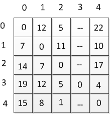
Table 2.1 — Table of distances

2.2 Deykctra algorithm

Adgoritm finds the shortest distance from one of the vertices of the graph to all others. The algorithm works only for graphs with no edges of negative weight and is widely used in programming and technology.
The essence of the algorithm will be discussed later. [3]
There is a directed graph G, which is depicted in Figure 2.1

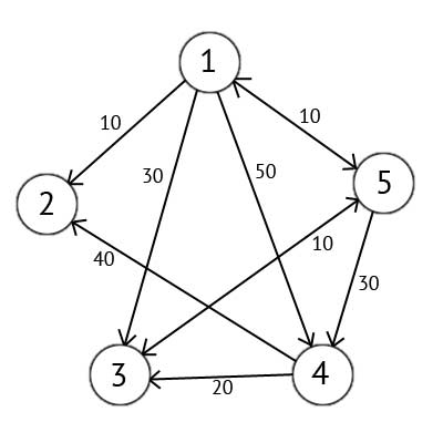
Figure 2.2 — A directed graph G
This graph, we can provide a matrix C:
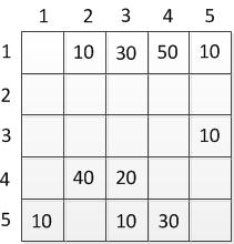
Table 2.2 — Matrix of a directed graph

We select the top one. This means that we seek the shortest routes from the top 1 in the top 2, 3, 4 and 5. This algorithm step by step through all the vertices of the graph and assign them labels that are known to the minimum distance from the top of the source to a particular vertex. Consider the example of the algorithm. Assign the 1st top mark of 0, because this node - the source. The remaining vertices to label equal infinity.

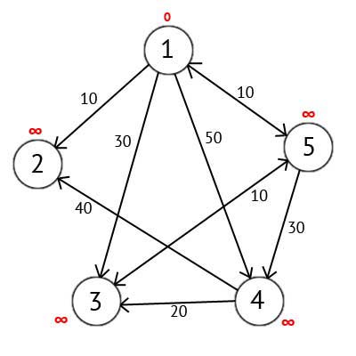
Figure 2.3 — A directed graph after the first step

Next, choose a vertex W, which has a minimum label and look at all the vertices in which the vertices of W is a path that does not contain vertices of intermediaries. Each of the peaks considered assign a label equal to the sum of the labels W and W long way from the top to the considered, but only if the amount received is less than the previous value of the label. If the amount is less, leaving unchanged the label.

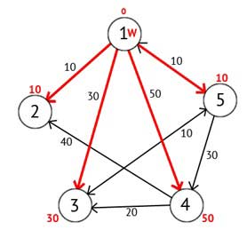
Figure 2.4 — A directed graph after the second step

Next, the top mark as visited W, and choose from not yet visited one that has the minimum value of the label, and it will be the next vertex W. In this case, the Vertex 2 or 5. If there are multiple nodes with the same label, it does not matter which of them can be chosen as W.

We select the top 2. From it there is no way of proceeding, then you can immediately point vertex as visited and move on to the next vertex with minimal label. At this time, only the tip 5 has a minimum mark. Consider all the vertices in which there is direct path out of 5, but are not yet marked as visited. Again, find the sum of the top label W and W of the edge weight in the current node, and if that amount is less than the previous mark, then replace the value of the label on the amount received.

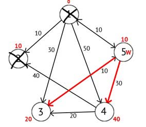
Figure 2.5 — A directed graph after the third step

Based on the pictures you can see that labels the third and fourth peaks are smaller, that is, found a shorter route to these peaks from the top of the source. Next, note the 5 th vertex as visited and select the next node that has the minimum label. Repeat all the above steps as long as there is not yet visited the summit.
After completing all the steps, we get the following result:

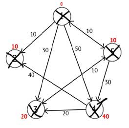
Figure 2.6 — A directed graph in the final step

3 Kalman Filter

To improve the signal quality must be filtered. Filtration is a data processing algorithm that removes the noise and the information signal which distorts utility. One of the most common filter is a Kalman filter.

Kalman filter — the filter algorithm is used in many fields of science and technology. It can be found in the GPS-receiver, smart sensors in a variety of control systems. It uses a dynamic model of the system. The algorithm consists of two repeating phases: prediction and correction. The first state in the prediction is calculated a next time (considering their measurement errors). In the second, the new information from the sensor adjusts the predicted value (also taking into account the inaccuracies and noise of this information):

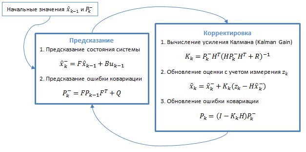
Figure 3.1 — General filter algorithm

3.1 Model of a dynamical system

Kalman filters are based on the sampled time-linear dynamic systems. State of the system is described by a finite-dimensional vector — the state vector. At each step of time linear operator acting on the state vector and transforms it into another state vector (deterministic change of state), added some vector of Gaussian noise (random factors) in the general case, the vector control, which simulates the impact of the management system.

When using a Kalman filter to obtain estimates of the state vector of the process by a series of noisy measurements necessary to present a model of the process in accordance with the structure of the filter — in the form of a matrix equation of a certain type. For each measure k of the filter must be in accordance with the procedure below to determine the matrix: the transition between the processes F_k; measurement matrix H_k; process noise covariance matrix Q_k; measurement noise covariance matrix R_k; in the presence of control actions — a matrix of coefficients B_k.

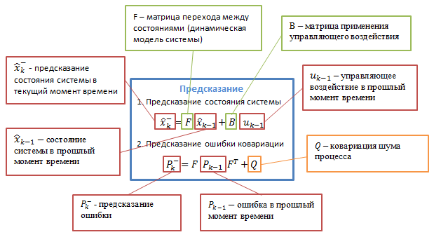
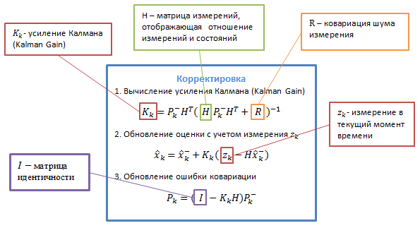
Figure 3.2 — Detailed description of the algorithm [9]
x_k = F_kx_k-1 + B_ku_k + w_k, where F_k — matrix evolution process / system that affects the vector x_k-1 (state vector at time k-1);
B_k — control matrix that is applied to the vector control actions u_k;
w_k — normal random process with zero mean and covariance matrix Q_k, which describes the random evolution of the system / process: w_k ~ N (0, Q).
At time k to be observed (measured) z_k of the true state vector x_k, which are connected by the equation: z_k = H_kx_k + v_k, where:
H_k — measurement matrix relating the true state vector and the vector of the measurements, v_k - white Gaussian noise measurements with zero mean and covariance matrix R_k: v_k ~ N (0, R_k).

The Kalman filter is a type of recursive filter. To compute an estimate of the current state of the system clock cycle it needs assessment (in the form of assessment and evaluation of errors in determining this status) in the previous cycle and the measurement of the current cycle. This feature distinguishes it from the packet filters that require a current measure of knowledge of the history of measurements and / or estimates. Next, by writing Xn | m going to understand the true estimate of x at time n with the measurements from the start of the work and the time m inclusive.

Pk | k — a posteriori error covariance matrix that specifies the assessment of the accuracy of this estimate of the state vector, and includes an assessment of the state of the calculated error variance and covariance, showing the relationship between the identified parameters of the system (in Russian literature often denoted Dk);
Xk | k — a posteriori evaluation of the state of the object at time k obtained from observations up to and including the moment of k (in Russian literature often denoted Xk, where X stands for "evaluation", and k - number of cycles at which it is received).

As the moving object will choose a ship whose motion is described by a system of differential equations subject to linear motion.

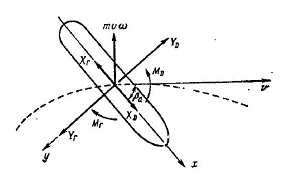
Figure 3.3 — model of the ship in the circulating pool. [8]
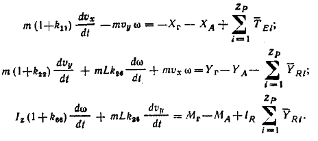
The model of the ship is described by the following system of equations:

4 Parallel Architecture

Currently, to improve the performance of computing systems are widely used different approaches. One of them is the use of multicore and multiprocessor architectures. [1]

4.1 Parallelism as a basis for High Performance Computing

Multiprocessor systems can be classified as follows:
SISD (Single Instruction Single Data) - single instruction stream, single data stream (sequential von Neumann computers). This class includes sequential computer systems that have one central processor that can process only a single stream of instructions executed sequentially. This is the usual scalar, single-processor systems. [10]

SIMD ((Single Instruction Multiple Data) - characterized by a single instruction stream multiple data stream but. This class includes single-processor, vector-pipelined supercomputers.
Another subclass of the SIMD-vector systems are the computers. Vector computers manipulate arrays of similar data, just as scalar machines process the individual elements of arrays. This is done through the use of specially designed vector CPUs. [10]

MIMD - computer architecture, which is used to achieve high-performance parallel computing. The peculiarity of this system is that the computer has multiple processors, which operate independently and asynchronously. Different processors at any time can execute commands on the various pieces of data. MIMD architectures are further classified according to the physical organization of memory, that is, whether the processor has its own local memory and accesses to other blocks of memory, using a switching network, or switching network connects all the processors to the shared memory. Based on the organization of memory, the following types of parallel architectures for distributed memory computers (Distributed memory) processor can access local memory, can send and receive messages on the network connecting the processors. Messages used for communication between the processors, or equivalently, for remote reading and writing memory blocks. In the idealized value of the network to send a message between two nodes in the network does not depend on the location as both nodes and the traffic network, but depends on the length of the message. [2]

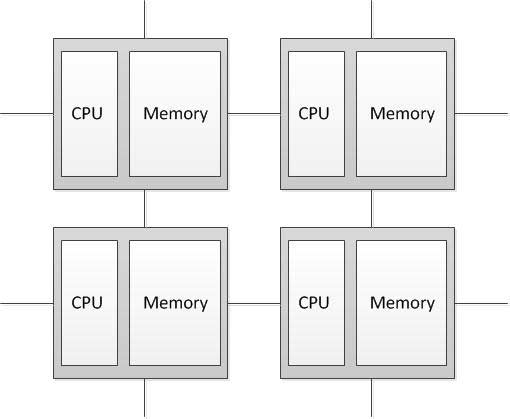
Figure 4.1 — Structure of the computer with distributed memory

4.2 Parallel GPU Architecture

Another version of the parallel architecture is the graphics processor (born graphics processing unit, GPU), which is a separate unit of personal computer that performs graphic rendering. Due to the pipelined architecture specialized they are much more effective in the processing of graphical information than typical central processor.

To speed up the application of the universal joint use of the GPU and CPU to perform calculations. GPU computing was invented by NVIDIA and quickly became the standard in the industry, which is used by millions of users around the world, and which was almost all manufacturers of computer systems.

CPU + GPU - system, which increases the computational power due to the fact that consist of multiple CPU cores optimized for sequential processing data while GPU consist of thousands of nuclei created for parallel data processing. Successive parts of the code are handled by CPU, and parallel portions - on the GPU.

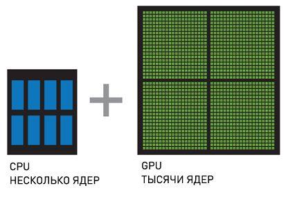
Figure 4.2 — CPU + GPU [6]

5 Approach and implementation

Parallel architectures have their own characteristics in the implementation of algorithms. Parallel programming is used to create programs that effectively use the computing resources through the simultaneous execution of code on multiple compute nodes. To create parallel applications using parallel programming languages and specialized systems for parallel programming, such as MPI and Cuda. Concurrent programming is more complicated than in a serial coding, and in its debugging.

5.1 MPI

MPI - the software interface for the transmission of information that allows you to exchange messages between processes that perform a single task. MPI is the most common standard for data exchange interface in parallel programming, its implementation, there are a large number of computer platforms. Used to develop programs for clusters and super computers. The primary means of communication between processes in the MPI is to pass messages to each other. Primarily focused on the MPI system with distributed memory, that is, when the costs of data transmission are great. The basic mechanism of communication between the MPI processes is the sending and receiving of messages. Message carries the transmitted data and information to enable the receiving party to carry out their sampling technique: [7]
1. sender - the rank (number per group) sender;
2. recipient - the rank of the recipient;
3. sign - can be used to separate different types of messages;
4. communicator - the code of the process group.

Transmit and receive operations can be blocked and not blocked. For non-blocking operation, the functions check availability and expectations of the operation.

5.2 CUDA

CUDA - hardware and software parallel computing architecture, which can significantly increase the computing performance by leveraging the GPU company NVIDIA. [5]
The architecture of the CUDA memory model is used grid, cluster modeling of flow and SIMD-instructions. Applicable not only for high-performance visual computing, but also for a variety of scientific computing using graphics cards nVidia. Scientists and researchers are widely used CUDA in various fields, including astrophysics, computational biology and chemistry, fluid dynamics simulation, electromagnetic interactions, computed tomography, seismic analysis, and more. In CUDA has the ability to connect to applications that use OpenGL and Direct3D. CUDA - cross-platform software for operating systems such as Linux, Mac OS X and Windows.

6 Results

Relevance of the use of super computers, and thus the parallel architecture in predicting the behavior of a moving object is the need to perform calculations of the parameters of the object, its trajectory path and behavior depending on external factors in the shortest possible time.

When forecasting the behavior of the moving object is critical speed calculations in connection with the need to improve the efficiency of these algorithms. This is a major and urgent task.

Source List

1. Parallel Computer Architecture: A Hardware/Software Approach (The Morgan Kaufmann Series in Computer Architecture and Design), Callifornia, 1999, 1025c
2. MIMD. Electronic resource. Access mode:
http://www.ccas.ru/paral/mimd/mimd.html
3. Deykctra algorithm. Electronic resource. Access mode:
http://habrahabr.ru/post/111361/
4. Floyd–Uorshell's algorithm. Electronic resource. Access mode:
http://urban-sanjoo.narod.ru/floyd.html
5. CUDA. Electronic resource. Access mode:
http://www.nvidia.ru/object/what_is_cuda_new_ru.html
6. CUDA Parallel Computing Platform. Electronic resource. Access mode: http://www.nvidia.com/object/cuda_home_new.html
7. Message Passing Interface Forum. Electronic resource. Access mode:
http://www.mpi-forum.org/
8. Ходкость и управляемость судов. Под ред. В.Г. Павленко. М.: Транспорт, 1991., с. 318.
9. Kalman filter. Electronic resource. Access mode:
http://habrahabr.ru/post/140274/
10. SIMD and SISD. Electronic resource. Access mode:
http://rudocs.exdat.com/docs/index-43961.html?page=13