ДОНЕЦКИЙ НАЦИОНАЛЬНЫЙ ТЕХНИЧЕСКИЙ УНИВЕРСИТЕТ

A new proximity sensor uses an RF field to sense near-field proximity with high precision.
G. Trummer, C. Kurzhals, R. Gehring, and D. Leistner
MTS Mikrowellen Technologie und Sensoren GmbH
At the moment, inductive, capacitive, optical, and ultrasound sensors are used to measure distance to objects in the proximity range. Inductive sensors work only with metal objects, the material and size of which must be known so that measurements can be carried out with sufficient precision (reducing factor). Inductive sensors mounted immediately adjacent to one another will affect one another, since the vision range of each sensor is 180°. Static and dynamic magnetic fields disturb the function of the sensor, and measurement precision fluctuates with temperature. With capacitive sensors, the object always serves as an intentional second capacitor plate and so both the material and size of the object must be known in order to reliably measure the distaэce to the sensor. In addition, measurement precision is affected by relative humidity, temperature, and electromagnetic fields. Optical sensors can be used only to a limited extent in an industrial environment, since they can no longer be

Figure 1. The ceramic RF resonator setup is shown with (G) or without (A) the electronics; the block diagram shows the signal processing electronics. (B) shows the front end. The electromagnetic wave enters the resonator through a coupling slot (C), and part of the wave is coupled out again through a second coupling slot (D). The broadband detector diode (E) determines its RF power. Adjusting the frequency using the oscillator (F) determines the resonance frequency detuning causing by an approaching object, enabling precise measurement of the object's proximity.


guaranteed to work properly in dirty conditions. The measurement precision of ultrasound sensors depends very largely on the ambient conditions, e.g., air humidity and temperature.

This article introduces the next generation of proximity sensors that avoid these disadvantages.

The Operating Principle

The operating principle (see Figure 1) is based on the frequency detuning of a cylindrical resonator filled with dielectric material. A weak electromagnetic field is generated at radio frequencies (5–6.5 GHz for an M18 size sensor) and coupled into the ceramic-filled cavity (the resonator). Some of this field leaves the cavity at the front; any object in front of this surface reflects the electrical field and couples it back into the cavity. The reflection influences the resonant frequency of the cavity; circuitry detects this frequency shift and electronics evaluate the signal.

The surface of this ceramic cylinder is gold-plated, except for the front end facing the object. The distance between this front end and the target is determined using the principle of a waveguide resonator. A part of the line is formed from a dielectrically filled waveguide short-circuited at one end. The other part is formed by the free space and a metallic or dielectric object located in front

Figure 2. The sensor's functional properties are outlined by a geometrical setup and a simplified equivalent circuit. The electromagnetic field in the dielectric resonator spreads out to the target. The distance to the target forms part of the resonance circuit and determines the resonance frequency.


of the sensor (see Figure 2). This free space line can be imagined, more or less, as a continuation of the waveguide metallization from an ideally magnetic conductor. The object accordingly forms the terminal resistance of the magnetic waveguide. If the distance between the sensor and measurement object (or the reactance of the measurement object) changes, this is associated with a change in the free space line and thus the resonance frequency. The measured resonance frequency is thus a function of the distance. In contrast to a radar sensor, however, the sensor must not radiate the electromagnetic field into free space. Through careful selection of the dielectric, it is possible to ensure that only an evanescent field (i.e., reactive power) can emerge from the waveguide. This behavior also determines the sensor’s maximum range.

The electromagnetic wave is fed into the resonator via a coupling slot on the gold-plated front end. Through a second coupling slot, a part of the electromagnetic wave is coupled out again and its RF power determined via a broadband detector diode. If an object now approaches the open front end of the resonator, the resonance frequency is detuned. This detuning is determined by changing the frequency of the oscillator, until resonance is detected through an RF power change at the detector diode. Then the frequency sweep of the oscillator is stopped immediately. The frequency that is now set corresponds to the resonance frequency, and the following resonance condition, as shown in Figure 2, applies, where Z1 is the wave resistance in the ceramic, Z2 is the wave resistance from sensor to target, ?1 is the propagation constant in the ceramic, ?2 is the propagation constant from sensor to target, l1 is the ceramic length, and l2 is the distance from sensor to target:

(1)

Solving for l2 this becomes:

(2)

The wave propagation occurs at the speed of light in the free space and in the ceramic. In comparison, the speed at which the target is approaching is negligible. Therefore highly dynamic target movements are measured with a precision of <1 µm. At slower target

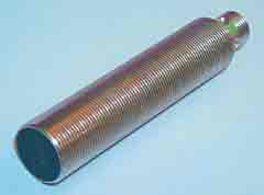
Figure 3. This is the sensor in a typical threaded barrel configuration.


approach speeds, higher measurement accuracy is achieved by averaging values (e.g., averaging 200 values leads to a repeatability accuracy of 200 nm).

Figure 1G shows the resonator with the assembled RF electronics. These are inserted into the threaded barrel and connected with the interface board as in standard inductive proximity sensors. Figure 3 shows the complete sensor in an M18 size.

RF Configuration of the Resonator
For propagation-capable modes, the surface currents Js=n?H may not be interrupted. Only in the TE0np modes do the currents flow parallel to the cover edge, without exception. The widest unambiguous range across the frequency is obtained with the TE011 mode, where the subscript denotes cylindrical coordinates (r, , and Z). To obtain clear resonance behavior, the loaded quality factor QL of the resonator (the measure of loss of a resonant circuit) must be large. This is achieved through loosely coupling the resonator using a horizontal magnetic dipole (HMD). The HMD can be realized through a slot in the metallized cover surface of the resonator. The field equations for the TE011 mode of a circular waveguide are:

(3)

where:

= resonant frequency
= permittivity
kc = cutoff wave number
µ = permeability

Physical Dimensions of the Resonator
The maximum resonance frequency is achieved when the waveguide is closed. This means, ideally, that the object should be conductive and should cover the front end of the sensor completely.

In this case, the length L of the circular waveguide filled with a dielectric is calculated for a given frequency fr as:

(4)

where:

r = 2f = resonant frequency
= permittivity of the dielectric
µ = permeability of the dielectric

For the resonator of the M18 sensor, ceramic is used with a dielectric constant r of ~37.5 and a diameter D of 12.7 mm. For a maximum resonance frequency of 6.5 GHz, the length L is selected as 5.5 mm.

Simulation of the RF Characteristics
The sensor’s RF characteristics are simulated using the computer analysis program CST–Microwave Studio, which is based on the finite integral method. This includes simulation of the electromagnetic characteristics for varying dielectric constant, physical size of the resonator, and environmental conditions. The specific analysis model derived allows the prediction of the electromagnetic characteristics in both time (transient mode) and frequency (intrinsic mode) domains.

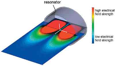
Figure 4 shows the electric field of the sensor for the selected TE011 mode.

Figure 4. The electrical field strength shows the sensor detection area in front of the ceramic RF resonator. Within this area the change in the resonance frequency decreases exponentially with increasing distance to the target. The change of the resonance frequency is at equidistant points in the near field of the sensor, e.g., at 1 mm in the megahertz region while it goes down to kilohertz in the far field, e.g., at 10 mm.

The longitudinal section illustrates the electric field strength for the case of an “open” resonator (without a target).

The logarithmic amplitude of the field can be used to explain the distance relationship shown in Figure 5.

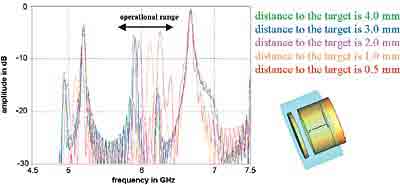
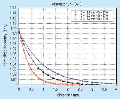
Figure 5. The quality factor of the operational resonance frequency band for the M18 sensor configuration is plotted for different target distances. Through loosely coupling the resonator with the transmit/receive part of the sensor by a horizontal magnetic dipole, a sharp resonance frequency line is achieved.

As the distance between the sensor and object increases, the part of the field that can be influenced by the object becomes smaller, as does the effect on the change in the resonance frequency. The propagation constant of the field ? becomes imaginary in the free space (since kc is >r2µ) and so the field subsides exponentially. The change in the resonance frequency also decreases exponentially with distance. The sensor becomes more selective as the distance decreases.

Figure 6 shows the simulation results for the sensor range over the normalized resonance frequency shift for three different resonator sizes.

Figure 6. The near field of the sensor detection range for three different sensor sizes is shown as a simulation result. In the absolute near field (<1 mm), the sensor has the greatest sensitivity.

The dielectric constant remains unchanged at 37.0. For a resonator with a lower dielectric constant, the gradient of the exponential descent is smaller and the range of the sensor increases. However, the measurement accuracy suffers under a smaller gradient.

Test Results

Figure 7 shows the measured values of the resonance frequency shift of the M18 sensor as a function of distance.

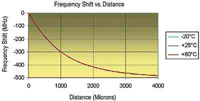
Figure 7. The detection range vs. frequency shift is shown for several field tests of the M18 sensor at different temperatures. Over a temperature range of 100°C the accuracy of the measured distance changes by <4 µm.

Temperature dependency of the sensor is avoided by using a temperature-compensated ceramic. Test results are plotted for temperatures of –20°C, 25°C, and 80°C; no visual deviation between the three curves is recognizable. The physical parameters of the sensor are as described before (r=37.5, D=12.7 mm, L=5.5 mm). The maximum resonance frequency occurs with a short-circuited resonator and is ~6.5 GHz with this sensor. The greatest sensitivity is achieved with short distances (objects close to the sensor); as the distance increases, the sensitivity steadily decreases, asymptotically approaching the limit value of the open resonator (lowest frequency). The frequency shift that can be reached here is ~500 MHz. The test results coincide exactly with the theory of Equation 1 and the simulation results of Figure 6.

EMC problems, such as those arising with inductive and capacitive sensors (e.g., caused by welding robots), do not occur since the working frequency of the sensor is in the gigahertz range. Environmental conditions such as dust, smoke, waste gases, and high relative humidity of the type occurring in normal industrial conditions do not affect the function of the sensor. All metals can be used as the target objects, and magnetic qualities are not necessary. To calculate the exact distance to the target, you must specify in your order whether the target is metal or dielectric; in the latter case the dielectric constant is required.

Further Applications
In general, the sensor can be used whenever extremely precise distance measurements are required, e.g., with wheel bearing monitoring in cars. By measuring the shift between the inner and outer ball socket, it is possible to determine the tangential and radial forces during driving. This means that the electronic stabilization program for cars can be dramatically improved. Further applications include measuring the thickness of metal sheeting, safety technology, quality assurance, plastic injection molding, and printing presses.

Availability
Samples of the precision optimized version (M18 size for metal targets) are available off the shelf for different accuracy and range settings (see Figure 12).

Figure 12.
Available Versions of the M18-Sized Sensor
Type Accuracy at Min. Range Accuracy at Max. Range Part Order No.:
Standard 6 µm at 0 µm
(0.23 mil at 0 mil) 80 µm at 4000 µm
(3.12 mil at 156 mil) 2012 M18 V1
High precision 4 µm at 200 µm
(0.156 mil at 7.8 mil) 40 µm at 2000 µm
(1.56 mil at 78 mil) 2012 M18 V2
Very high precision 1.5 µm at 200 µm
(0.0585 mil at 7.8 mil) 2 µm at 600 µm
(0.078 mil at 23.4 mil) 2012 M18 V3
Ultra high precision 800 nm at 200 µm
(0.0312 mil at 7.8 mil) 1 µm at 400 µm
(0.039 mil at 15.6 mil) 2012 M18 V4
Note: Other accuracy and range settings are possible on request without hardware changes.

CST–Microwave Studio is a trademark of CST Gesellschaft fьr Computer Simulationstechnik, Darmstadt, Germany.

A Typical Application: Friction Stir Welding

Figure 8. One typical application for the proximity sensor is in friction stir welding of aluminum sheets. This picture shows the robot configuration.


In the future, aluminum sheets in aircraft construction will be joined using friction stir welding. The welding tool here is a round, rotating disk that uses its kinetic energy as it penetrates the metal sheets to melt the plates at the point of entry. The quality of the welding process depends on the depth of penetration of the tool, its constant speed of rotation, and the degree of wear. Figure 8 shows the welding robot, and Figure 9 shows the sensor assembly. Figure10 shows the sensor’s time signal during welding, and Figure 11 shows the associated spectrum. In Figure 10, we can clearly see the individual phases of the welding process over time:

A) The measurement object appears within the range of detection of the sensor
B) The rotating tool comes into contact with the component for the first time
C) The rotating tool pulls back again
D) The rotating tool penetrates the component between C and D and starts the welding movement
E) The rotating tool reaches the end position
F) In the forward movement, the rotating tool is lifted

Figure 9. Here we see the sensor mounted on the robot.

Figure 10. This plot shows the sensor signal in the time domain during the welding process. The sensor is controlling the penetration depth of the tool during welding and guarantees a reliable welded joint.

The spectrum in Figure 11 clearly shows the speed of the tool at 49 Hz as the principal maximum level, with higher harmonics reaching higher frequencies.

Figure 11. The plot of the sensor signal in the frequency domain is shown. By controlling the rotational velocity of the tool and its harmonics the welding process can be optimized and tool wear recognized.

The amplitudes of these harmonics serve directly to determine the degree of the tool’s degree of wear. Very marked harmonics indicate a high degree of tool wear.

--------------------------------------------------------------------------------
G. Trummer is President and CEO, C. Kurzhals is Program Manager for proximity sensors, and R. Gehring and D. Leistner are Senior Microwave Design Engineers, MTS Mikrowellen Technologie und Sensoren GmbH, Ottobrunn, Germany; +49 89-6-07-2-36-85, gtrummer@mts-web.de.

For information in the U.S., please contact Peter Schmitz, MTS Communication & Sensors, Inc., Chicago, IL, 800-620-2126, pgschmitz@earthlink.net.

Первоисточник: www.sensorsmag.com