|
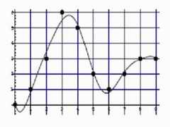
Source:"http://www.ii.metu.edu.tr/~ion528/demo/lectures/6/2/index.html" Digital image acquisition (digital sampling, the Nyquist frequency, aliasing, convolution) Digital image acquisition1 Digital sampling In chapter 1 we already mentioned that when acquiring an image of a real scene it is discretized in two ways: sampling and quantization. Figure 1 shows sampling and quantization of a one-dimensional signal on a uniform grid1. The signal is sampled at ten positions (x = 0, ..., 9), and each sampled value is then quantized to one of seven levels (y = 0, ..., 6).
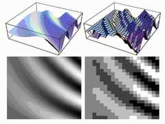
Sampling and quantization of images is done in exactly the same way, except that sampling is now done in more than one dimension. An example is shown in figure 2. Here, we see a continuous signal of two variables (top left), and the corresponding image with signal strength converted to grey values (bottom left). On the right, the signal is shown after sampling on a discrete grid and quantization of the grey values onto five levels. Note: even though this is a book about image processing, we will often use examples taken from one-dimensional signal processing wherever this simplifies matters.
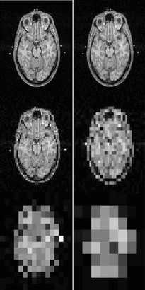
By simply looking at figure 2, it is clear that the digital picture is not a very good representation of the original. Obviously the density of the sampling grid and the number of levels we choose in the quantization are important quality factors. These factors are called resolution: the spatial resolution equals the number of pixels used, and the intensity resolution equals the number of grey levels used. In digital images, both types of resolution are finite. The effect of lowering the spatial resolution can be seen in figure 3. There is another kind of resolution called the optical resolution, which is the smallest spatial detail a visual system can see. Optical and spatial resolution are often used without their adjectives in texts, and what type of resolution is meant should be determined from the context.
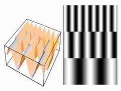
2 The Nyquist frequency If we sample an image, is it possible to make the image exactly the same as the original? And if so, how many samples are necessary? Before we can answer these questions, we need the concept of spatial frequency. The frequency of a sinusoid is defined as the number of cycles it makes per unit length. For example, the family of functions f(x) =sin(ax) has frequency a/2П . Figure 3.4 shows three sinusoids of different frequency and the corresponding image. There is a relationship between spatial frequency and the level of detail in images: a high level of detail corresponds to a high frequency, and a lack of details corresponds to low frequencies. A high level of detail is made up of relatively large contrast, i.e., the image intensity cycles fast from dark to light and vice versa, just like a high frequency sinusoid does. This relationship between frequency and image detail is at the heart of many image processing applications and will be explored further in the chapter on the Fourier transform.
We already noted that, in a digital image, the spatial and intensity resolution are finite. Hence the finest detail that can be represented is limited, and the range of spatial frequencies occurring in the image is also limited. This implies that the number of samples we must take of an image in order to exactly reproduce all the details is also finite. This observation is linked to spatial frequency by the sampling theorem: “To capture the highest frequencies (i.e., the smallest details) of a continuous image, the sampling rate must be
Note: many books use “band” terms when discussing frequencies. If the frequency has a limited range, it is called bandlimited. The range of frequency values itself is called the bandwidth. If we sample an image below the Nyquist frequency, details will be lost. Oversampling, on the other hand, will not increase the level of detail: all of the details are already captured when sampling exactly at the Nyquist frequency. Example: consider the following line taken from an image:
The pattern has a frequency of 1/2 per pixel –i.e., there are 2 in a pattern cycle–so the Nyquist frequency is
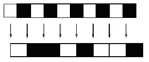
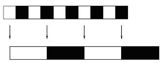
Если уменьшить частоту дискретизации до 1/3 за пиксель, то полученный образ будут иметь детали отсутствовавшие в подлинном изображении:
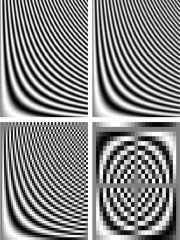
3 Aliasing The phenomenon occurring at the end of the example above is called aliasing: if we sample an image at a rate that is below half the Nyquist frequency, high frequency patterns in the original are translated to lower frequency patterns that are absent in the original image. In the example above, we see that a pattern with frequency 1/2 per pixel is mapped to a pattern with frequency 1/6 per pixel. Example: figure 8 shows another example of aliasing.
We sampled the function f(x; y) = 4 Sampling and convolution Until now we have assumed that we can sample an image with infinite precision. In practice this is an impossibility, since practical imaging devices cannot have an infinite precision. For example: if we use a camera to take samples of some infinitely small image location (x,y)y), then the camera will gather its sample in a small neighborhood around (x,y). There is in fact another reason why sampling with infinite precision is impossible: cameras need the energy from incoming light rays to detect these rays. Even if it were possible to point the camera with infinite precision at only the infinitely small point ((x,y), the energy of the incoming light rays would be reduced to zero, and we would detect nothing. There is a tradeoff here: on the one hand we would like our sampling to be as precise as possible, so a small sampling area, but on the other hand the sampling area cannot be too small, or it will not give off enough energy for proper detection. UpSource: |
 or faster, where
  equals the highest frequency occurring in the original image.
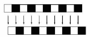
 on the domain в области
 which has decreasing frequency as we move from the top to the bottom line: frequency 25 per line on the top line, and frequency 1 per line on the bottom line. The function was sampled four times using different sampling frequencies. The aliasing effect at the lowest sampling frequency is so strong, that the high image frequencies at the top of the image get mapped to the same frequencies as the low ones at the bottom of the image.