Theme of abstract: Research and development of specialized software for modeling self-oscillations
Contents
Introduction
Relevance of the work
Objectives and expected scientific innovation
Expected practical results
1. Architecture modeling programs
1.1 The modular structure of programs, mathematical modeling of dynamic systems
1.2 Architecture of mathematical modeling programs with the core flow management model
1.3 GUI programming mathematical modeling of dynamic systems
2. Modeling systems of equations in MATLAB
Conclusion
References
Introduction
There are a lot of math programs. They can be divided on two groups:
- A powerful calculator for static calculations (Matcad, Mathematica, Maple).
- Specialized solvers for simulation of dynamic processes (DyMoLa, Dynast, Multisim, VisSim, MBTY, MVS, Simulink).
The user needs to determine the sequence of mathematical functions, which should be evaluated by mathematical kernels. The difference is manifested in the fact that if you use programs calculators user should only rely on a single calculation of a programmed sequence of functions, while using dynamic solvers can use the opportunity of repeated calculations. Thus, on the one hand, if at your disposal program, a calculator, then you need to know a huge amount of methods to reduce the number of mathematical operations [1]. On the other hand, when using dynamic solvers for the solution of problems in the forehead, will have to seriously get a computer processor several billions of mathematical operations on two or even ten seconds.
Computers, of course, not invented for office applications. The brain does not developed for remembering of a large number of formal or rigidly algorithmic techniques that were developed before the advent of computers in order to reduce the amount of computation. These facts explain the considerable interest in leading teachers to the program of mathematical modeling of dynamic systems. However, limitations in the availability of such programs, the desire of producers to hide the technology of their operation, plus a nationwide love for "calculator" hinder their widespread use, generate mistrust of him, which ultimately affects their quality.
Relevance of the work
Broadening the range of scientific and technical problems facing the computer technology requires a highly effective means of simulation. Use of parallelism leads to resolution of problems synthesis of computing processes with minimal overhead in the implementation on regular OS. In this regard, the task of designing an optimal schedule for modeling dynamic systems is actual today.
Objectives and expected scientific innovation
Improving the digital part of the complex in the solution of problems of modeling hard dynamic systems and the expand the class of tasks.
Expected practical results
1. Analysis of planning processes, real-time of computing in modern operating systems;
2. Algorithm development planner without interruption of the computational process using the theory of the schedule;
3. Software implementation of the test model of self-oscillations on the basis of the developed specialized software.
1. Architecture modeling programs
1.1 The modular structure of programs, mathematical modeling of dynamic systems
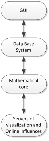
The modular structure of the simulation, almost unchanged (see Fig. 1):
- Graphical user interface. Oriented to person and is responsible for presenting mathematical model as understood by the wider community. This may be a block-diagrams, physical principle, hybrid maps of states, etc.
- Database management system is responsible for storing objects drawn by the user model and the required transformation of the structure of the repository.
- Mathematical core takes on the main computational load and, in the cycle, according to a given program, guided by the willingness of the arguments, and in rare cases of dispute (the occurrence of which can always be avoided) the priority of mathematical operations, provides execution flow of mathematical functions.
- Servers of visualization and Online influences provide the interface between a functioning core of the mathematical and the user.
|
Figure 1 - The modular structure of the simulation programs
|
Developers modeling programs to create their products do not adhere to modern technologies of modularization (COM, CORBA) and prefer to do everything yourself. All presented in Fig. 1 modules can not be simply self-contained, and has traditionally been considered independent software products. Mathematical core - this is the most simple and easy to create a module. Creating a full-fledged vector graphics editor like Visio or CorelDraw, or a relational database engine - it's not a task for companies with a staff of 3 .. 10. That effort expended to solve these minor problems, have ruined not one company, and lose from this user.
Over the past ten years the situation has not changed in favor of the developers described the position of simulation programs. Auxiliary modules created by competing with each other by third parties, are widely available, provide the required mechanisms to integrate with other software complexes, and continuously improved by professionals in their field.
1.2 Architecture of mathematical modeling programs with the core flow management model
Whatever may have been different modeling programs, variations in architecture their mathematical kernels rather severely limited opportunities compilers of high level languages. Mathematical kernel must support 100 to several thousands of mathematical functions. Of course, you want to formalize the interface to configure and manage the mathematical kernel as to cope with such a huge number of functions, using their manual call impossible.
1.3 GUI programming mathematical modeling of dynamic systems
Graphical User Interface - this is the "weak spot" programs of mathematical modeling of dynamic systems. Let's try to deal with the fact that it can understand the Russian language specialist at a modest English term diagram, if you want to use it to describe the system model at any level in graphic form:
1. Flowcharts, or about a dozen named directed graphs.
2. Schemes physical principle of electrical, magnetic, thermal, hydraulic, acoustic, mechanical, rotary, etc. chains of energy conversion.
3. Hybrid maps of state or pulsed stream graph, the transition states.
4. Graphs algorithms programs.
5. Block diagrams, functional diagrams.
6. And much more.
Diversity is impressive. But the purpose of transferring not shock the reader's imagination and to bring to the idea that the task of creating a graphical user interface is not simple and does not meet qualifications of the developers of modeling programs. The end user must understand that without cooperation of efforts of several companies that will not solve the problem (user demand creates supply). The task of the qualitative mapping of the foregoing, on any scale, on any device I / O can be overcome only if a vector graphics editor - it is their direct problem. Additional requirements for the applicant for its implementation is open object architecture and the availability of documentation.
Clearly visible, only two modeling techniques: structural modeling and multiple domain physical modeling. To support the structural model is required solver of systems of differential equations and block diagrams [2]. To support multiple domain physical simulation requires an iterative solver of systems of algebraic-differential equations and the physical principle scheme [3]. Other types of graphs either not effective or are the ancestors of directed and undirected graphs respectively. Simulation is event-driven is not a new modeling technique, but complements a set of techniques called switching and synchronizing fragment patterns in the simulation, thus providing a software flow control.
2. Modeling systems of equations in MATLAB
For simplicity of modeling systems of equations we take the environment MATLAB. We simulate a system consisting of 3 equations, 2 of which represent the Van der Pol, the third is the relationship between  and
and  . The system has the form:

To solve this system were created 2 files:
- vdpol.m will contain a function to compute the system
function xdot = vdpol(t, x)
w=[1 1];

T=1-x(1)^2-x(3)^2;

xdot = [x(2);...

-w(1)^2*(x(1));...

x(4);...

-w(2)^2*(x(3)+T)];

end
- vdpol_LANCH.m will contain a command to call a function vdpol.
t0=[0 10];           %Simulation interval

x0 = [0 0.3 0 0.7];  %Initial conditions

[t, X] = ode45('vdpol', t0, x0);

[m,n] = size(X)

plot(t, X)

figure; surfc([1:n], [1:m], X)

shading interp

colorbar
For research use the following initial values:

We carry out several measurements with different values  .
.
1.  .
.
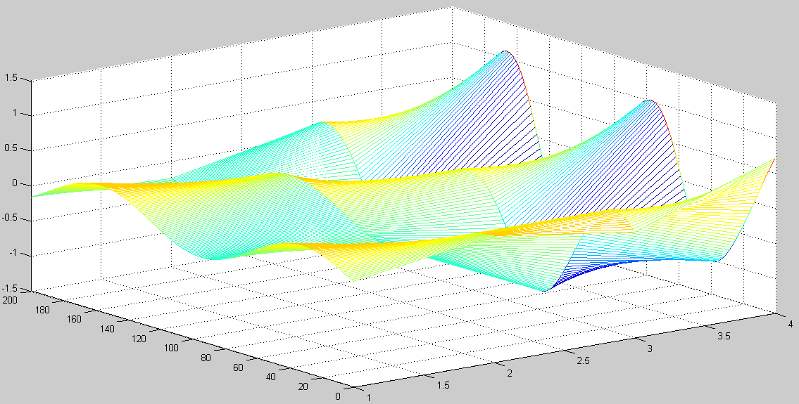
After performing the functions we obtain the following time schedule and three-dimensional model.
|
Figure 20 – Timeline for
|
|
Figure 21 – 3D model for
|
2.  .
.
After performing the functions we obtain the following time schedule and three-dimensional model.
|
Figure 22 – Timeline for
|

|
Figure 23 – 3D model for
|
3.  .
.
After performing the functions we obtain the following time schedule and three-dimensional model.

|
Figure 24 – Timeline for
|

|
Figure 25 – 3D model for
|
4.  .
.
After performing the functions we obtain the following time schedule and three-dimensional model.

|
Figure 26 – Timeline for
|

|
Figure 27 – 3D model for
|
Conclusion
In this paper, the MATLAB environment was modeled system of equations of Van der Pol consisting of three equations with two unknowns. During the simulations using different input data. All simulated systems of equations have timelines. The same for systems of equations are represented by their 3D models.
In writing this abstract master's work is not completed yet.
References
1. Клиначёв Н. В. Обзор архитектурного построения программ математического моделирования динамических систем. - Челябинск, 2004.[электронный ресурс]. – Режим доступа: www/URL:http://model.exponenta.ru/simkernel.html
2. Клиначёв Н. В. О структурном кризисе в методике преподавания блока дисциплин связанных с расчетом цепей преобразования энергий. - Челябинск, 2003.[электронный ресурс]. – Режим доступа: www/URL:http://model.exponenta.ru/lectures/sml_06.htm
3. Клиначёв Н. В. Введение в технологию моделирования на основе направленных графов. - Челябинск, 2003.[электронный ресурс]. – Режим доступа: www/URL:http://model.exponenta.ru/lectures/sml_02.htm
4. Клиначёв Н. В. Введение в технологию мультидоменного физического моделирования с применением ненаправленных графов. - Челябинск, 2003.[электронный ресурс]. – Режим доступа: www/URL:http://model.exponenta.ru/lectures/sml_03.htm
5. Хайрер Э., Нёрсетт С., Ваннер Г. Решение обыкновенных дифференциальных уравнений. Нежесткие задачи. М.: Мир, 1990. 512 с.
6. Хайрер Э., Ваннер Г. Решение обыкновенных дифференциальных уравнений. Жесткие и дифференциально-алгебраические задачи. М.: Мир, 1999. 685 с.
7. Козлов О.С., Медведев В.С. Цифровое моделирование следящих приводов. В кн.: Следящие приводы. В 3-х т. Под ред. Б.К. Чемоданова. М.: Изд. МГТУ им. Н.Э. Баумана, т. 1, 1999, с.711-806.
8. Shampine L.F., Reichelt M.W. The MATLAB ODE Suite // SIAM J. on Scientific Computing. Vol. 18. 1997. № 1. P. 1-22.
9. Bogacki P., Shampine L.F. A 3(2) pair of Runge-Kutta formulas // Applied Mathematics Letters. Vol. 2. 1989. № 4. P. 321-325.
10. Hosea M.E., Shampine L.F. Analysis and implementation of TRBDF2 // Applied Numerical Mathematics. Vol. 20. 1996. № 1-3. P. 21-37.
11. Скворцов Л. М. Адаптивные методы численного интегрирования в задачах моделирования динамических систем // Изв. РАН. Теория и системы управления. 1999. № 4. С. 72-78.
12. Скворцов Л. М. Явные адаптивные методы численного решения жестких систем // Математическое моделирование. Т. 12. 2000. № 2. С. 97-107.
13. Скворцов Л. М. Диагонально неявные FSAL-методы Рунге-Кутты для жестких и дифференциально-алгебраических систем // Математическое моделирование. Т. 14. 2002. № 2. С. 3-17.


