
Abstract
Contents
- Introduction
- 1. Theme urgency
- 2. Goal and tasks of the research
- 3. Overview of research and development
- 3.1 Overview of international sources
- 3.2 Overview of national sources
- 3.3 Overview of local sources
- 4. The finite element method as the basis of calculations in modeling
- 5. Using the constraint programming in CAD systems
- Conclusion
- References
Introduction
CAD, or computer–aided design systems, are digital platforms, created to increase the efficiency of engineers, because nowadays few people prefer paper drawings to electronic ones. They are widely used in almost many areas of industrial and construction activities.
Nowadays computer technologies are developing rapidly, and CAD systems are getting more and more high-quality abilities to design objects and their modeling under conditions of physical and temperature loads, as well as calculation of aero- and hydrodynamics of the designed models. Thus, improving the accuracy of modeling is one of the main tasks of CAD modernization.
1. Theme urgency
CAD systems are divided into subsystems, and the one responsible for modeling objects is CAE - Computer-Aided Engineering. CAE is a set of software products that can give the user a description of how in reality it will be behave like a computer-developed product model. With the help of CAE, an engineer can accurately assess the performance of a product without resorting to significant time and money costs. In their work, CAE use various mathematical calculations: finite element method, finite volume method, finite difference method.
It often happens that the excessive accuracy of the mathematical calculations used can be the cause of an error when modeling an object. This, in turn, in real conditions can cause malfunction of the product or even breakage of the latter. In this regard, methods of programming in constraints have been developed that allow the machine to find the right solution to the problem that arises. The approach proposed in this paper uses the methods of interval mathematics, which allows us to take a fresh look at the ways of setting constraints.
2. Goal and tasks of the research
The purpose of the work is to design and develop an application that implements modeling of a given object using the finite element method modified for constraint programming.
Main tasks of the research:
- Analysis of CAE system development methods.
- Implementation of the constraint programming method.
- Justification of the requirements for the system being created, as well as for the input parameters entered by the user.
- Description of the program algorithm.
- Evaluation of the effectiveness of using constraint programming when working with different models.
Research object: implementation of the CAE system modified for constraint programming research.
Research subject: the effectiveness of the use of programming in constraints within the framework of the CAE subsystem of modern CAD systems.
3. Overview of research and development
3.1 Overview of international sources
Christoph M. Hoffmann in his work "Constraint-Based CAD" examines the current stage of CAD development and highlights the available ways of setting constraints in product design, their advantages and disadvantages. The author also suggests the idea of a CAD based on setting constraints.[1]
Nikhil Somani, Andre Gaschler, Markus Rickert, Alexander Perzylo and Alois Knol in their article "Constraint-Based Task Programming with CAD Semantics:From Intuitive Specification to Real-Time Control" describe the possibility of controlling robots using a CAD software package and inter-relational geometric constraints.[2]
3.2 Overview of national sources
In the work "Object-oriented programming in constraints: a new approach based on declarative data modeling languages" Semenov V.A., Ilyin D.V., Morozov S.V., Sidyaka O.V. consider and discuss a new systematic approach to the implementation of object-oriented programming in constraints based on the use of declarative data modeling languages.[3]
Narinyani A.S. in his work "Introduction to Subdefinition" introduces the method of underdetermined models proposed by the author in the 80s of the last century for the presentation and processing of not fully defined knowledge.[4]
3.3 Overview of local sources
The topic of constraint programming in modern CAD systems is of interest to the masters of Donetsk National Technical University.
R.E. Komarichev was researching on the development of systems implementing the finite element method in various CAD models, whether physical, thermal or aerodynamic effects on the product, followed by the output of simulation results. He also identified several potential sites for optimization in his master's thesis.[5]
S.D. Krilevich and A.V. Grigoriev in the article "Development of a system for the automated solution of computational CAD problems based on the method of programming in constraints" considered the methods of implementing an instrumental system for solving programming problems in constraints in various formulations arising in the process of problem-oriented CAD. The problem statements of the developed programming system in constraints, as well as the data structures of its model, were determined. A general dynamic computational model capable of providing a solution to the tasks set has been developed.[6]
4. The finite element method as the basis of calculations in modeling
One of the most used modeling methods in modern CAD is the finite element method (FEM). It is a numerical method for solving partial differential equations, as well as integral equations arising in solving problems of applied physics. The method is widely used to solve problems of deformable mechanics solid state, heat transfer, hydrodynamics, electrodynamics and topological optimization.
As already mentioned, the FEM is now one of the most popular tools for studying the characteristics of engineering structures subjected to various loads. Traditional methods involving strict theoretical justification, can be used only for a limited class of tasks and special load conditions. They often need modification, and it is necessary to control their applicability to solve the problem. The designers' lack of confidence in the reliability of the results obtained forces them to increase the maximum loads, which leads to the inclusion of additional fastening sections in the design, overspending of materials and an increase in the total cost of the product.[7]
The essence of the finite element method lies in its name. The domain in which the solution of differential equations is sought is divided into a finite number of subdomains, and in each the type of approximating function is randomly selected from them. In the simplest case, it is a polynomial of the first degree. Outside of its element, the approximating function is zero. The values of the functions at the boundaries of the elements (in the nodes) are the solution of the problem and are unknown in advance. Coefficients of approximating functions are usually searched from the equality condition of the value neighboring functions on the boundaries between elements, i.e. in nodes. Then these coefficients are expressed in terms of the values of the functions in the nodes of the elements. A system of linear algebraic equations, in which the number of equations is equal to the number of unknown values in the nodes on which the solution of the original system is sought, is directly proportional to the number of elements and is limited only by the capabilities of the computer. Since each of the elements is connected to a limited number of neighboring ones, a system of linear algebraic equations it has a sparse appearance, which greatly simplifies its solution.[8]
After dividing into finite elements, further calculations are carried out for individual finite elements, each of them contributes to the strength characteristics of the part. The points bounding the element are called nodes, which together with the lines passing through them form a finite element grid.
For two-dimensional areas, the most commonly used elements are in the form of a triangle and a quadrilateral. At the same time, the elements can have both rectangular and curved borders, which makes it possible to approximate the border of any shape with a sufficient degree of accuracy. For three-dimensional areas, the most commonly used elements are in the form of a tetrahedron and a parallelepiped, which can also have straight and curved boundaries.[7]
Obviously, different finite element models are used for different tasks. Different types of elements and coordinate functions are also used. In case you need to consider for a more detailed model, the density of the finite element grid can be increased by reducing the size of the latter.[9]
For a long time, the widespread use of FEM was hampered by the lack of algorithms for automatically dividing the area into "almost equilateral" triangles (the error, depending on the variation of the method, is inversely proportional to the sine of either the sharpest or the most obtuse angle in the partition). However, this task was successfully solved (the algorithms are based on Delaunay triangulation), which made it possible to create fully automatic finite element CAD systems.
We will demonstrate an example of the operation of the finite element method. To do this, we use some cylindrical object and simulate elastic deformation for it. As you can see, the object it is divided into a set of rectangular elements, colored blue in the initial state, which indicates zero deformation. After the start of deformation modeling, the coloring of some elements changes - in this way it is possible to determine which parts of the product are most deformed in this experiment.
Fig. 1 – Deformation simulation demonstration
(animation: 4 frames, 608 kilobytes)
5. Using the constraint programming in CAD systems
It can be difficult for a CAD user to anticipate all the factors that will affect the simulated object in real life, and therefore it is necessary to reduce the accuracy of modeling. In this case, you need to use the constraint programming method.
Constraint programming is inherently as declarative as possible and is based on a description of the problem model, not an algorithm for solving it. The model is specified in the form an unordered set of relationships that correspond to the relationships that exist between the task parameters. These relations, called "constraints", can take the form of equations, inequalities, logical expressions, etc.
In the most general form, the problem statement in the programming paradigm in constraints is formulated as follows. Let the variables x1, x2 ..., xn be the areas of values which are sets (X1 , X2 , ..., Xn), constraints Ci (x1 , x2 , ..., xn), i=1, k. It is required to find sets of values (a1 , a2 , ..., an) (ai belongs to Xi), which would satisfy all the constraints at the same time.[10]
This formulation of the problem is called the constraint satisfaction problem, and various algorithms and methods are used to solve it. In particular, the problem of satisfaction constraints can be formulated as a system of equations with numerical parameters, and standard numerical methods can be used to solve it. This is suitable enough for the solution modeling tasks, but not always effective for real-world conditions, since not all data types can be used in such tasks.
One of the most developed and practically significant approaches related to constraint programming is subdefinite models.
The technology of subdefinite models stands out among other approaches for computing power, versatility and efficiency. In fact, it is the only technology, which allows us to solve the constraint satisfaction problems in the most general formulation.
The following concepts are the basis of the subdefinite models unit:
- A subdefinite variable is some non-empty subset containing a denotation value inside itself, which remains unknown due to lack of information; an available estimate of the real value;
- A subdefinite extension is any finite system of subsets of a set X, closed with respect to the intersection operation and containing the entire universum and an empty set. For the same universum, there may be several different undefined extensions.[11]
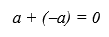
Some properties of ordinary operations change significantly in the corresponding subdefinite extensions. As an example, consider the well-known property of additive operations over numbers (integer or real) that the sum of any number and its inverse is equal to a single zero element.
Let the subdefinite extension of the set of numbers be an interval subdefinite extension, and the corresponding subdefinite extensions of the minus (*-) and plus (*+) operations are defined according to the known rules of interval arithmetic. Thus, the undefined extension of the unary minus has the following form:
![[aLo, aUp] = [-aUp , -aLo]](images/diss_pic2.png)
The subdefinite extension of addition (a = b *+ c) is calculated this way:
![[aLo, aUp] = [bLo + cLo , bUp + cUp]](images/diss_pic3.png)
In this case, the subdefinite extension of the expression (a + (-a) = 0) has the following form:
![[aLo, aUp] *+ (*-[aLo, aUp]) = [aLo, aUp] *+ [-aUp, -aLo] = [aLo + (-aUp), aUp+ (-aLo)] = [aLo - aUp, aUp - aLo ]](images/diss_pic4.png)
Thus, if the lower and upper bounds of an subdefinite number do not match, the interval [aLo - aUp , aUp - aLo] only contains a zero element, but it is not exactly equal to it.
Drawing a conclusion from the above, in undefined models it is very important in what form the conditions of the problem are presented, which can be a significant addition to the finite element method.
Conclusion
Summing up the described statements, the use of underdetermined model technology will allow using not only discrete, but also interval values of variables in constraint satisfaction problems. It is assumed that the inclusion of interval mathematics in the FEM can improve its performance in some simulated situations.
This master's work is not completed yet. Final completion: June 2023. The full text of the work and materials on the topic can be obtained from the author or his head after this date.
References
- Christoph M. Hoffmann. (2005). Constraint-Based Computer-Aided Design. Journal of Computing and Information Science in Engineering 5(3):182. DOI:10.1115/1.1979508 [Link]
- Nikhil Somani, Andre Gaschler, Markus Rickert, Alexander Perzylo, Alois Knol. (2015). Constraint-Based Task Programming with CAD Semantics: From Intuitive Specification to Real-Time Control. IEEE/RSJ International Conference on Intelligent Robots and Systems (IROS)At: Hamburg, Germany. DOI:10.1109/IROS.2015.7353770 [Link]
- Семенов В.А., Ильин Д.В., Морозов С.В., Сидяка О.В. Объектно-ориентированное программирование в ограничениях: новый подход на основе декларативных языков моделирования данных [Электронный ресурс] // КиберЛенинка - научная электронная библиотека. - Режим доступа: [Link]
- Нариньяни А.С. Введение в недоопределенность [Электронный ресурс] // КиберЛенинка - научная электронная библиотека. - Режим доступа: [Link]
- Комаричев Р.Е. Анализ технологий программной реализации метода конечных элементов [Электронный ресурс] // Портал магистров ДонНТУ. — Режим доступа: [Link]
- Крилевич, С.Д., Григорьев, А.В. Разработка системы автоматизированного решения вычислительных задач САПР, основанной на методе программирования в ограничениях [Электронный ресурс] // Электронный архив Донецкого Национального Технического Университета (г. Донецк). - Режим доступа: [Link]
- Чернышов Д.Н., Грищенко О.С., Григорьев А.В. Использование метода конечных элементов для физических расчетов в САПР // Материалы VI Международной научно-технической конференции «Современные информационные технологии в образовании и научных исследованиях» (СИТОНИ-2019). – Донецк: ДонНТУ, 2019. - С. 347-352.
- Чернышов Д.Н., Григорьев А.В., Воробьев Л.О. Расширение функциональных возможностей подсистем моделирования и инжиниринга (CAE) в современных САПР. // Материалы студенческой секции X Международной научно-технической конференции «Информатика, управляющие системы, математическое и компьютерное моделирование» (ИУСМКМ -2021). –Донецк: ДОННТУ, 2021. - С. 100-104.
- Основные этапы решения задач методом конечных элементов - САПР конструктора машиностроителя [Электронный ресурс] // Студенческие реферативные статьи и материалы. - Режим доступа: [Link]
- Ушаков Д.М., Телерман В.В. Системы программирования в ограничениях (обзор) // Системная информатика: Сб. науч. тр. Новосибирск: Наука, 2000. Вып.7: Проблемы теории и методологии создания параллельных и распределенных систем. С. 275—310.
- Нариньяни А.С. Недоопределенные модели и операции с недоопределенными значениями. – Новосибирск, 1982. – 33с.