
Abstract on the topic of the graduation work
Content
- Introduction
- 1. Purpose and goals of the system
- 2. Existing systems
- 3. Tasks to perform
- 4. Mathematical statement of the problem
- 5. Methods and Algorithms
- 5.1. Japanese Candlestick Analytical Method
- 5.2. Last Value method
- 5.3. Moving average method
- 5.4. Linear Regression
- 5.5. Extreme Gradient Boost (XGBoost)
- 5.6. Long-term short-term memory (LSTM)
- 5.7. Time series decomposition
- 5.8. Holt Method — Winters, Brown. Exponential Smoothing
- Conclusions
- List of sources
Introduction
Nowadays, many people buy and sell stocks, currencies, futures, options, and so on. Also, many are just learning it. People come to the exchange and leave, making history. Obviously, the main goal is to make money. But in addition to money, a trader receives a lot of other moral pleasures. Freedom from superiors, the ability to choose when and where to work. The exchange gives you the opportunity to make money with your head. The game on the stock exchange combines many activities at once. A lot of people have made their fortunes thanks to the exchanges, but there are a lot of people who who say: "Only the owner of the casino wins in the casino." It's not quite right, you have to think with your head, find patterns and this is bearing fruit and one can come to the conclusion that price movements are quite predictable. Few people know that the physicist Newton was a big fan of playing the stock market. He didn't play very well. Even completely unsuccessful. Once, after a major loss, he uttered the famous phrase: – I can predict the movement of cosmic bodies, but I cannot predict the madness of the human crowd (price movements and the behavior of speculators). The famous "tulip fever" that happened in Holland in the 17th century also went down in history. Things got to the point that ships and estates were given away for a handful of tulip bulbs ... Therefore, the tool with which it was possible to assume the movement of prices would be more than ever useful for traders on the stock exchange.
1. The purpose and goals of creating the system
The web-based system will be used to assist corporate traders as well as individuals
whose activities are related to trading on the stock exchange in any form (spot, futures, options).
The system is created to simplify the trading process by providing trading recommendations.
The developed WOS is intended for:
- demonstration of information about trading pairs in the form of a chart, with a choice of timeframes, showing the price in real time.
- Providing trading recommendations based on forecasting methods.
The goals of creating the “VOC analysis of exchange trading pairs”:
- Increasing the profitability of a trader's work using the created tool.
2. Existing systems
There are quite a few systems representing options for price movements on exchanges, but these options are mostly paid.
Existing options:
- Charts from ru.tradingview.com, in this system it is possible to create your own plug-ins for forecasting, and use other people's, however, a paid subscription is required for full use, besides, good plug-ins are purchased separately.
- eSignal — a Windows based application that uses JavaScript as the basis for a scripting language that programmers and traders can use to create custom indicators. This, in fact, includes eSignal users in a database from which programmers can be drawn to write indicators.
- Wealth—Lab — A program designed for the technical analysis of financial markets, developed in the early 2000s by Dion Kurczek. Since 2004 it has been owned by Fidelity Investments. Users can create and test trading strategies for stocks and futures.
- PIAdviser — advisor-analyst, the full name of the system is PersonalInvestmentAdviser, created as a tool for analyzing stock exchange data, predicts price dynamics, generates trading signals (MICEX, COMMODITIES, NYSE, FORTS, NASDAQ, ETF, FOREX), helps to teach trading—technologies, teaches you how to create your own trading system.
3. Tasks to perform
- To analyze the subject area, existing methods and models for forecasting prices on the stock exchange;
- Definition of parameters, restrictions and general mat. productions;
- The choice of languages and means for the implementation of the task;
- The choice of methods for the implementation of the task;
- Development of forecasting algorithms;
- Checking the accuracy of models on a series of tests and determining their effectiveness.
4. Mathematical statement of the problem
Price values are a time series at discrete times t=1,2,…,T. Previous price values are presented as follows Z(t) = Z(1), Z(2),…, Z(T). At time T, it is necessary to determine the values of the process Z(t) at time points T+1, T+2, ..., T+P. The moment of time T is called the forecast moment, and the value of P — lead time (the time for which it is necessary to make a forecast).
Formulas used for the task:
- Moving Average formula p: $$\overline{Z}(t) = {1\over P} \cdot (Z(t)+Z(t-1)+...+Z(t-p-1))$$
- Average absolute deviation of the true value from the predicted one: $$\overline{E} = {1\over P} \sum_{t=T+1}^{T+P} [\varepsilon_t] \rightarrow \min$$
- Definition of a time series, at a point in time: $$x_{t+1}=m_{t-1}+{1\over n}\cdot (x_t-x_{t-1})$$
- Average absolute forecast error: $$MAPE = {1\over n} \sum_{t=1}^{n} [{{x_t-\widetilde{x_t} }\over{x_t}}] \cdot 100%$$
- Mean squared error: $$MSE = {1\over n} \sum_{t=1}^{n} ({x_t-\widetilde{x_t} })^2$$
5. Methods and algorithms
Time series forecasting algorithms are most often considered in the economic field, where they are used to predict quotes, market volumes, financial indicators, etc. One of the most interesting time series for forecasting is, perhaps, the prices of stock pairs. The following methods and algorithms have been chosen that have already been used previously, related to forecasting prices on stock exchanges:
- Japanese candlestick analysis method;
- Last Value method;
- Moving Average or Moving Average [MA];
- Linear regression;
- Extreme gradient boost (XGBoost);
- Long Short Term Memory (LSTM);
- Time series decomposition;
- Method Holt – Winters, Brown. Exponential smoothing.
Metrics of mean squared error (RMSE) can be used to evaluate the effectiveness of these methods and mean absolute percentage error (MAPE). For both indicators, the lower the value, the better the forecast.
5.1. Japanese Candlestick Analytical Method
Japanese candles are a type of chart used in the technical analysis of the stock market. It consists of rectangular figures - candles, each of which corresponds to a certain time interval.
Visual representation of the chart during trading with possible price movement in fig. 1.
Figure 1 - Japanese candlesticks
(animation: 12 frames, repeat-loop, 55 kilobytes)
(1-upper shadow, 2-close price, 3-candle body, 4-open price, 5-lower shadow)
A candlestick consists of two elements - the body and the shadow. The boundaries of the body show the level of the opening price and closing at a given time interval. And the borders of the upper and lower shadows show the maximum and the minimum price for the same interval. There are two types of candles - bullish and bearish. The bullish candle reflects the rise in prices for the specified interval and its body is not painted over. On color charts, a rising candlestick is green and a falling candlestick is red. In an ascending (bullish) candle, the upper boundary of the body indicates the closing price, and the lower opening price. A descending (bearish) candle characterizes a price fall and its body is painted in dark color. On such a candle, the upper boundary of the body indicates the opening price, and the lower one indicates the closing price. The most accurate forecast is given by the “hammer” and “hanged man” candles. They signal a chart reversal. Both candles have a small body and a long shadow. "Hammer" is located at the bottom of the chart and indicates a trend reversal upwards, and the Hanged Man is at the top of the chart, indicating a downward trend reversal.
5.2. Method Last Value
In the Last Value method, the forecast was set to the last observed value, i.e. current adjusted closing price as the adjusted closing price of the previous day. It is the most cost-effective forecasting model and is commonly used as a benchmark to compare more complex models. The disadvantage of this model is that it does not give any guarantees, but only is a standard for comparison with the data obtained by other methods.
5.3. Moving Average or Moving Average [MA]
The simplest and fastest forecasting option — calculate the average estimate of the last values of the series. In a recommendation problem, it is usually important that the last values in the series have more weight. Entering the coefficients depending on the distance of the date from the current one, we will get a weighted model: $$y_t = {1\over k} \sum_{i=1}^{k} y_{t-i}$$ $$y_t = {1\over k} \sum_{i=1}^{k} w_{k-i}y_{t-i}$$ For example, for w = ( 0.4, 0.05, 0.05, 0.05, 0.05, 0.3, 0.1) the highest recommendation value would be play the same day of the week a week ago and also in the last 2 days. Time series analysis using the sliding method The average is used, as a rule, in short-term forecasting. With insufficient data, the moving average method useless. And the projection on the future of old schemes is not always justified. Impossibility to take into account the impact random factors — this is another shortcoming of the moving average method[1].
5.4. Linear Regression
Linear regression is a linear approach to modeling the relationship between the dependent variable and one or more independent variables. In this case, linear regression was used, to fit a linear regression model to previous N values to use this model for predicting values for the current day. An example of linear regression that makes it clear the relationships between variables. Linear regression can give an approximate price movement, however, this method has a drawback, it will not give an idea of the price if the analysis is done on lower time frames (temporary price change on the site less than an hour) [2—3].
Visual display of linear regression is shown in Figure 2.
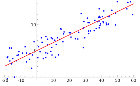
Figure 2. Linear regression
5.5. Extreme Gradient Boost (XGBoost)
Gradient boosting is the process of iteratively transforming weak learners into strong learners. The name XGBoost refers to an engineering goal to expand computing resources. for improved tree algorithms. Since its introduction in 2014, XGBoost has proven to be very a powerful machine learning technique and is typically the go-to algorithm for many competitions on machine learning. The obvious use cases are adjusted closing prices. for the last N days, as well as the volume for the last N days. The disadvantages are that this method gives the analysis not very fast [4].
5.6. Long Short Term Memory (LSTM)
LSTM is a deep learning technique designed to deal with the problem of vanishing gradients, occurring in long sequences. The LSTM has three elements: an update gateway, forgetting gateway and exit gateway. The gates of renewal and forgetting determine whether each element of the memory cell is updated. The output gate determines the amount of information displayed in the form of activations to the next level. Following is the LSTM architecture. In the case of currency rate forecasting, two layers of LSTM modules and an intermediate layer are used, to avoid overfitting [5—6].
Scheme of the LSTM method is shown in Figure 3.
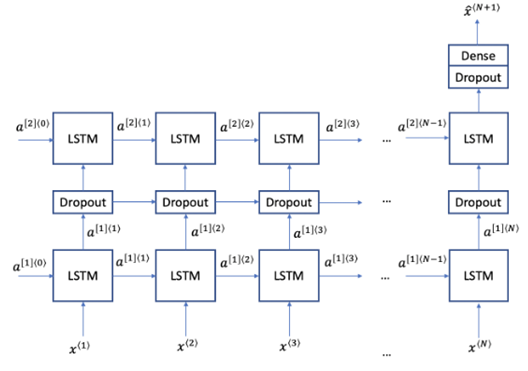
Figure 3. Schematic of the LSTM method
5.7. Time series decomposition
The quality of recommendations can be influenced by many cyclical factors, such as matching day of the week, date, precedence of holidays, etc. The classic and most complete forecasting model is as follows: $$Y=T*(S_1*S_2*S_3...S_n)*R$$
where: T — trend — a general trend of increase or decrease, depending, for example, on the popularity of the application; Si— seasonal components, which may be several, — for example, fluctuations in popularity depending on the time of year, day of the week, time of day; R— residuals (noise) — random fluctuations in values that are difficult to predict;
5.8. Holt Method — Winters, Brown. Exponential Smoothing
Extracting the components of a time series can be a difficult task, especially if if we do not know what kind of periodicity can be observed in the original data. However, there are methods to automate this task. A compromise between simple methods for calculating the average and more complex decomposition are methods of exponential smoothing. Within the framework of this approach, three models are widely known [8]:
- Simple dithering (Brown model)
- Double smoothing (Holt model)
- Triple smoothing (Holt — Winters model)
Simple smoothing is essentially a weighted average of the last 2 elements of the series.
Double exponential smoothing takes into account both the change in trend and fluctuations in residual values around this trend. In these formulas, we calculate the prediction of the change in residuals (l) and trend (d). The final value of y — the sum of these two quantities. This model is especially useful for predicting recommendations, because it allows you to take into account weekly (or daily) fluctuations without complicated manual settings.
$$r_t=ay_t+(1-a)(r_{t-1}+d_{t-1})$$ $$d_t=b(r_t-r_{t-1})+(1-b)d_{t-1}$$ $$y_{t+1}=r_t+d_t$$
A more complex — triple smoothing, which also takes into account seasonal fluctuations. This model is applicable if there is a sufficient amount of data and it is good there are seasonal changes (for example, in addition to daily fluctuations, there are also weekly fluctuations)
$$r_t=a(y_t-s_{t-L})+(1-a)(r_{t-1}+d_{t-1})$$ $$d_t=b(r_t-r_{t-1})+(1-b)d_{t-1}$$ $$s_t=g(y_t-r_t)+(1-g)s_{t-L}$$ $$t_{t+m}=r_t+md_t+s_{t-L+1+(m-1)modL}$$
Conclusions
The outcome of the presented methods will be decided to implement some of the methods for complex application, different methods will be used in different cases.
Methods will be used to check the quality of the used value: Mean Absolute Forecast Error (MAPE) and Mean Squared Error (MSE).
At this stage of the master's work, the goal and objectives for systems, a comparative analysis of existing systems was carried out. Were determined mathematical methods on the basis of which the functionality of the program will be implemented. Structure developed subsystems.
When writing this essay, the master's work has not yet been completed. Final Completion: May 2023 of the year. The full text of the work and materials on the topic can be obtained from the author or his supervisor after specified date.
List of sources
- Moving average method. [Electronic resource]. — Access mode: https://journal.open-broker.ru/trading/method-skolzyashej-srednej/....
- Seber J. Linear Regression Analysis Moscow: Mir, 1980. — 456 p.
- Kuprienko N.V. Statistical methods for studying relationships. Correlation and regression analysis., 2008. — 105 p.
- Gradient boosting. [Electronic resource]. — Access mode: https://ru.wikichi.ru/wiki/Gradient_boosting....
- LSTM – neural network with long short-term memory. [Electronic resource]. — Access mode: https://neurohive.io/ru/osnovy-data-science/lstm- nejronnaja-set/....
- Gafarov F.M., Galimyanov A.F. Artificial neural networks and their applications. Kazan, 2018. — 121 p.
- Electronic textbook on statistics from StatSoft. [Electronic resource]. — Access mode: URL: http://www.statsoft.ru/home/textbook/default.htm.. ..
- Time series in forecasting. [Electronic resource]. — Access mode: https://habr.com/ru/post/477206/....