
Attention!
At the time of writing this abstract, the master's work is not yet complete. Final completion: June 2024. Full text of the work and materials on the topic can be available from the author or his scientific advisor after the specified date.Forecasting the stock exchange quotation rate based on statistical data of the financial market using modern modeling methods
Introduction
Existence within the framework of the modern economic system is conditioned by multiple risks. Fluctuations in exchange rates, changes in supply and demand in various areas, various internal and external factors of an economic and political nature certainly affect both the entire system as a whole and its individual components at all levels. The need to form a strategy of action in conditions of this kind of uncertainty certainly actualizes the task of modeling these processes for all market participants – from countries for which the dynamics and predictability of changes in the exchange rate of the national currency determines the level of confidence of the population and entrepreneurs in the government of the country, to directly entrepreneurs of different levels and individuals for whom the dynamics of exchange rates determines the vector of investments and market strategies
Herewith, the reliability and durability of the models being developed comes to the fore as part of the planning task – the more accurate the model's forecasts, the longer-term forecast it returns, the more detailed a strategy can be formed by one or another market participant.
Purose and objectives of the study, the planned results
The purpose of this study is to identify the instrumental area and form a vector for the development of further research in the field of developing methods that can increase the predictive accuracy of models used in analyzing market behavior.
Basic concepts and definitions
The forecasting methods and techniques used in the context of finance can be classified according to the following parameters [1]:
- Based on the assessment: qualitative (as a rule, these are expert assessments based on judgments and conclusions) and quantitative (based on the calculation of numerical indicators)
- According to the information component: static (formalized) and intuitive.
Thus, taking into account the requirements for the universality of methods within the framework of the task of predicting the behavior of the system, the object of this study will mainly be quantitative formalized methods, the main source of information for which will be the history of the asset price, presented in the form of time series.
Time series
Time series (dynamics series) are sets of time–varying values of a certain indicator, grouped in chronological order [2]. As a rule, they are sequential sets of values $y_{1},y_{2},...,y_{n}$, also called levels of a series
, each of the levels has a certain point in time in accordance $t_{1},t_{2},...,t_{n}$
The classification of time series is very diverse. They are divided according to a variety of characteristics [2], for example:
- According to the form of representation of levels: on the series of absolute and average indicators, series of average values;
- By the nature of the time series: moment and interval;
- According to the time distance between the levels of the series: equally spaced and unequally spaced;
In this context, the most significant classification parameter is the nature of the random process, which divides the series into stationary and non-stationary.
Stationarity
A random process is strictly stationary (stationary in the narrow sense) if its finite-dimensional distributions are invariant with respect to the time shift, i.e. if its multidimensional probability density of arbitrary dimension $n$ does not change with simultaneous shift of all time segments $t_{1},t_{2},...,t_{n}$ by the same amount $\tau$[3][4]:
$\displaystyle{ p(x_1, x_2, ..., x_n, t_1, t_2, ..., t_n)=p(x_1, x_2, ..., x_n, t_1+\tau, t_2+\tau, ..., t_n+\tau), \tau\in\mathbb{N}} $
This factor largely determines which methods will be used during the analysis of the time series. This is due to the fact that most algorithms, on the basis of which various statistical criteria are built, spectral and correlation methods are always based on the constancy of mathematical expectation and variance, which is precisely a consequence of stationarity [3]. Moreover, since this property is decisive in the context of time series, it is precisely this property that is indicated in many sources as the definition of stationarity, thus expanding the introduced concept. Thus, in a broad sense, the definition of stationarity is as follows: a random process $x(t)$ is called stationary if its mathematical expectation and variance are constant in time, and the autocovariance function depends only on the difference of arguments [4]:
$\displaystyle{ m_x(t)=m_x=const, D_x(t)=T_x=const }
$\displaystyle{ K_x(t_1,t_2)=K_x(t_2-t_1)=K_x(\tau) }
An important note here is that in practice, a purely theoretical definition of the stationarity of a random process is not applicable. The hypothesis of the stationarity of the initial time series is verified using some statistical criteria that allow us to estimate with some confidence how much the characteristics of the time series satisfy the criterion of stationarity (for example, KPSS-test).
In practice, time series rarely turn out to be stationary, while stationary series are much better studied. The behavior of such series is more predictable, therefore it is easier to analyze and, most importantly, forecast [3], therefore, if possible, a procedure for reducing to stationarity is performed, the first and most important stage of which is the allocation of the trend component [6], after which, including using spectral analysis methods, the remaining ones are isolated The deterministic components of the time series model are cyclic and seasonal.
Time series models
All time series are based on a random process, which can be characterized in various ways: by describing some of its statistical characteristics, such as a distribution function, or by constructing some characteristic model of it [7].
В There are a very large number of ariants of models simulating such processes. One of the most common models is the so-called additive model, which characterizes the process as the sum of some deterministic ($q$) and random ($\xi$) component, which is also often called noise:
$\displaystyle{ A(T)=q(t)+\xi(t) }
Along with additive models, there are obviously multiplicative as well as mixed models in which both additive and multiplicative components are present at the same time:
$\displaystyle{ M(t)=q(t)\xi(t) }
$\displaystyle{ y_t(t)=M(t)+A(t) }
In addition, for stationary time series, there are a number of models describing them through a mathematical relationship between subsequent and previous values of the time series, as well as, in some cases, their noise. Such models are called autoregressive and can be reduced to the following formula:
$\displaystyle{ y(t_i)=f(t_{i-1},t_{i-2},...)+g(a_i,a_{i-1},a_{i-2})+\xi(t_i) }
Trend, cycle and seasonality
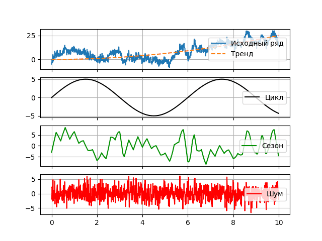
The deterministic component of the time series $q$ can be any arbitrarily complex mathematical function. The subclass of the model depends on the way it is divided, but in general, all models somehow operate with the following components: trend, seasonal and cyclical:
$\displaystyle{ q(t)=\tau(t)\circs(t)\circp(t) }
Trend ($\tau$) is some general trend observed over a long period of time. It is usually described by a simple monotone function of time [8].
The presence of a seasonal component ($s$) is associated with the presence of factors in a random process, the influence of which is determined by some periodicity (day of the week, month, year). As a rule, it is associated with some factors that occur in real life – such as weekends, holidays, harvest time, vacation time, etc. A special property of the seasonal component is the possibility of its floating character – the possibility of change over time, therefore they are called quasi-periodic [7].
The cyclic (periodic) component ($p$) is a non-random function with a pronounced trigonometric component that determines long periods of cycle change [9].
When analyzing time series, seasonal components are called quasi-periodic components of high frequency, while cycles are much more resistant to changes in longer-term components. At the same time, within the framework of one model, there may be several seasonal and cyclical components, and the relationship can be described by various relationships. Thus, for example, the general form of additive can be represented as the following expression:
$\displaystyle{ y(t)=\omega_\tau\tau(t)+\omega_s\sum_{j}s_j(t)+\omega_p\sum_{k}p_k(t)+\xi(t) }
where $\omega_\tau, \omega_s, \omega_p$ are the coefficients of presence or absence, taking exclusively the values 1 and 0.
The bifurcation point
When analyzing and calculating the trend component, it is important to remember that the system that generates a random process may be influenced by various internal and external factors, as a result of which the nature of its trend may change significantly.
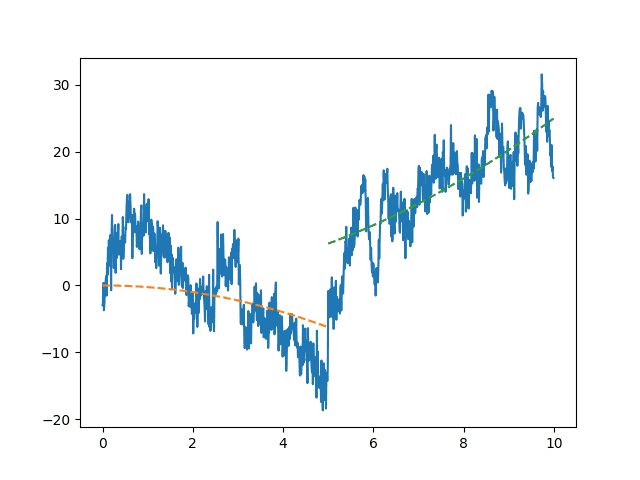
At the same time, extrapolation methods can accurately describe behavior within a single process, but at the same time they are not suitable at the time of their change [10]. Thus, one of the stages of the study of the time series is the search for the so-called bifurcation points
- time points in the studied series corresponding to a sharp change in the behavior of the system. In the intervals between the bifurcation points of the system, its behavior is predictable and stable, determined by the above-described factors.
Spectral analysis
After identifying the trend component of the deterministic part of the series, it becomes necessary to determine various periodic and quasi-periodic components of it, and in this case spectral analysis methods can be a serious help [11], allowing to identify hidden cyclic patterns in time series. At the same time, many time series models (Seasonal decomposition, SARIMA) to one degree or another assume that the researcher knows some parameters of the frequency characteristics of the series, which makes spectral analysis methods a powerful tool for processing time series.
There are quite a few methods of spectral analysis and they are all based on one idea – they transfer data from the value/time plane to the amplitude/frequency plane, thereby bringing to the fore the frequency characteristics of the series.
Neural network modeling
Neural network technologies deserve special mention in the context of time series modeling. An important aspect of these algorithms is their ability to generalize – neural networks in the learning process are able to find non-trivial connections within the data, and therefore increase the predictive ability of the model.
Recurrent neural networks. This type of algorithm is well suited for processing sequences [12]. The main idea of such neural networks, unlike the perceptron, is that the output of the neural network on the next element of the sequence depends on previous results.
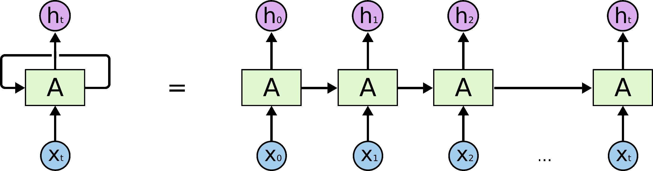
Due to their structure, it can be said that recurrent neural networks in a general sense are representatives of autoregressive models, since they display the relationship between time-spaced levels of a time series.
However, recurrent neural networks still have a number of disadvantages: the problem of explosion and decay of the gradient and the problem of parallelization. Due to the fact that in the process of calculations there is a repeated repetition of multiplications by the same value of weights, gradients either tend to infinity or to zero, which makes it difficult to obtain information from states far away in time [13]. This problem is solved by making certain changes to the structure of the model. However, the problem of parallelization arises as a consequence of the neural network architecture itself: calculations cannot be parallelized, since each subsequent internal state of the system depends on the previous one.
Abandoning the recurrent model, these problems are solved by neural network transformers, the main idea of which is that tokens pass through layers in parallel with each other, interacting with the help of the inner layer of Multi-head attention. This is a special layer that allows each input token to interact with others using the attention mechanism
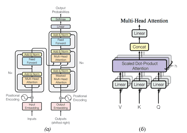
Vectors and a$Query$ number of pairs $(Key, Value)$are fed to the input of this layer. Each of them is transformed by a linear transformation, after which the scalar product is calculated$Query$ with all $Key$ in turn, processed using a logistic function and summed into a single vector with $value$. Its difference from the attention-s that were previously encountered in other works is that several such layers are trained in parallel (in the figure – $h$). After that, the result is concatenated again, processed using a trainable linear transformation and returned.
From the point of view of time series forecasting, such a multi–layered
mechanism allows you to process the sequence from different aspects - random filling of the initial weights is quite enough to direct the search for patterns along different paths. In addition, such a mechanism allows you to design multimodal systems capable of simultaneous processing of different types of data.
Justification of the direction of further development
Thus, in order to increase the accuracy of modeling financial processes, it is necessary to approach the problem comprehensively, increasing accuracy at all stages of time series analysis and modeling.
Search for bifurcation points
Since the behavior of the system changes unpredictably at bifurcation points, it is necessary to exclude their influence on the analyzed series by excluding the corresponding trend components. However, in many cases, visual analysis does not allow us to unambiguously indicate the presence of such points in a series. Hence, there is a need for a certain algorithm that allows you to find with high reliability the moments of change of processes that control the behavior of a series, as well as being able to confirm the presence of these points.
The algorithm for finding bifurcation points is based on replacing time series segments with a mathematical model and comparing the models of these models. At the same time, any model that is deterministic for the initial and predicted time values can act as a trend. [10].
Since it is assumed that the found bifurcation point divides the series into two independent segments, it can be argued that in order to find the optimal trend for the forecast, further search for trend break points should and should be carried out in the area lying to the right on the timeline relative to the bifurcation point.
ТThus, the algorithm for finding bifurcation points of a time series can be described as follows. Suppose there is a time series $y(x):(x_i, y_i), i=0,1,2,...N$, as well as an assumed model having $f(x)$ degrees of freedom. In this case, for each $k$ it is necessary to calculate:
$\begin{eqnarray} \overline{y_l}=f(x_i),i \in \lbrack 1;n_1 \rbrack \\ \overline{y_r}=f(x_i),i \in \lbrack n_1;N \rbrack \end{eqnarray}$
Having obtained, as a result, $n_1\in[k-1;N-(k-1)]$ potential bifurcation points and two series models for each of them, evaluating which using the distance metric, it is possible to determine which of the models is best suited, minimizing the distances found. For example:
$\begin{eqnarray} SS = \sum_{i=1}^{n_1-1}{(y_i-\overline{y_l}(x_i))}^2+\sum_{i=n_1+1}^{N}{(y_i-\overline{y_r}(x_i))}^2+\frac{2y_n_1-\overline{y_l}(x_i)-\overline{y_r}(x_i)}{2}\\ SS \to min \end{eqnarray}
In this case, the square of the distance was used as a metric, however, it should be mentioned that it is not universally the best, the list of metrics is quite diverse [16][17]. The value $2k-1$ found in this way will correspond to the bifurcation point of the time series when using the $n_1$ model at the specified interval.
Next, using statistical tests (for example, Fisher's F-test), it is necessary to determine the statistical significance of the resulting partition by comparing the ratio of the variance of the entire $f$ series and the total variance of its two segments $\sigma_{\mbox{ряда}}$ with the critical value $ \sigma_{\mbox{ступ}} $
$F_{\mbox{кр}}$
$\displaystyle{ \sigma_{\mbox{ступ}}=\sqrt{\frac{\sigma_1^2n_1 +\sigma_1^2n_1}{N-1}} }}$
$\displaystyle{ F = \frac{\sigma_{\mbox{ряда}}^2}{\sigma_{\mbox{ступ}}^2} }$
The fulfillment of inequality (14) in this case determines the statistical significance of the partition with the confidence probability $\displaystyle{ F > F_{\mbox{кр}} }$ specified in the definition of $F_{\mbox{кр}}$ – in this case, the process of searching for the bifurcation point is repeated for $\alpha$, otherwise $i \in \lbrack n_1;M \rbrack $ is relied on for the model $ \overline{y}=f(x_i), i \in \lbrack 1;N \rbrack $ of the entire series and the algorithm completes its work.
Spectral analysis
Spectral analysis is one of the most effective methods for identifying causal relationships between the components of the studied processes. Applying the principles of spectral decomposition of the measured functions into individual spectral components, it is possible to isolate significant information even under the influence of interference [18]. Based on the idea of decomposing a function in a certain frequency range, this group of methods can help researchers to accurately estimate the periodic and seasonal components of a time series model.
It is worth noting that, despite the wide variety of spectral analysis tools, the main focus of this section is on one specific group of methods, namely, the wavelet transform. This is due to their general versatility: this type of transformation implements a compromise solution between resolution in the time and frequency spectra. In addition, the wavelet transform unfolds a series in three-dimensional space amplitude/time/ frequency
, which allows you to clearly identify time components localized in time, and the possibility of reverse synthesis of the series allows you to transform data at the decomposition stage.
Thus, three directions of the applicability of spectral transformations in modeling the behavior of a time series can be determined: visual analysis of the spectral component, the use of noise reduction for data preparation, and decomposition modeling.
Visual selection of the frequency components of the series
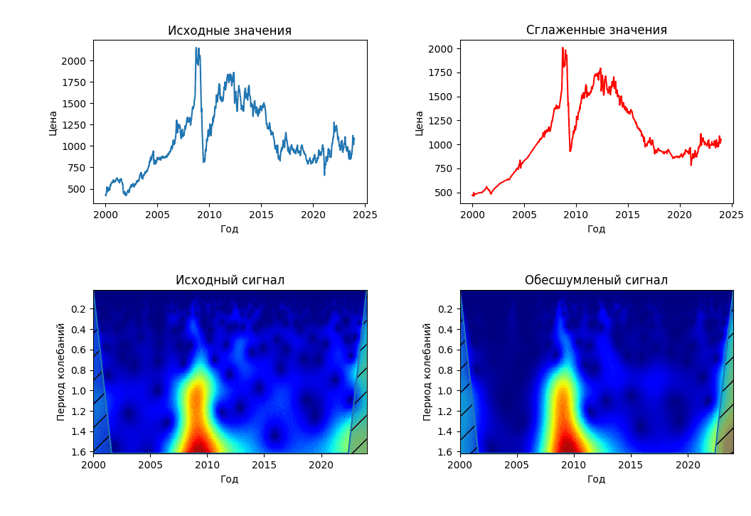
In essence, this direction is a direct application of wavelet analysis to a time series. By constructing a series diagram using a continuous wavelet transform, it becomes possible to visually evaluate periodic components:
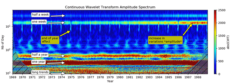
The continuous wavelet transform, unfolding a series of amplitude/frequency/time
space, allows you to visually assess the frequency components, the time of their appearance and disappearance, which allows you to describe them approximately, forming some model, which can be further refined using various fitting methods.
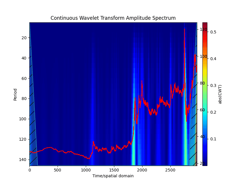
In addition to the method described in the previous section, the bifurcation points of the series will be quite clearly visible on the scalogram – at the moments of trend change, clearly defined peaks will be visible on it, affecting if not all, then most frequencies (Fig. 7).
Using noise reduction
For most signals, their low-frequency component is the most important part because it can be used to identify the signal. The high-frequency component, in turn, carries the outlines of the signal. If you delete it in the signal, it will change, but its main behavior will remain recognizable. However, if you remove a large number of low-frequency components of the signal, it will become unrecognizable. In wavelet analysis, approximations are studied on large scales, low-frequency components and details are studied on small ones.
For noise reduction, this method uses thresholding [19] (threshold data processing), a technique for studying signals containing noise, which decomposes the original signal into a wavelet spectrum, which is further processed.
A certain value of the filtering coefficient $k$ is selected, which determines the degree of smoothing of the values and the corresponding degree of thresholding $\Delta$, which is usually calculated using the formula:
$\displaystyle{ \Delta=kY_{max} }$
where $Y_{max}$ is the largest amplitude value in the spectrum.
Thus, values less than $\Delta$ in the spectrum are replaced by 0, and values higher or equal to it are compressed in the direction of 0 by $\Delta$. With hard thresholding, values less than $\Delta$ are replaced by 0, while larger values remain unchanged.
After that, the original signal is synthesized back:
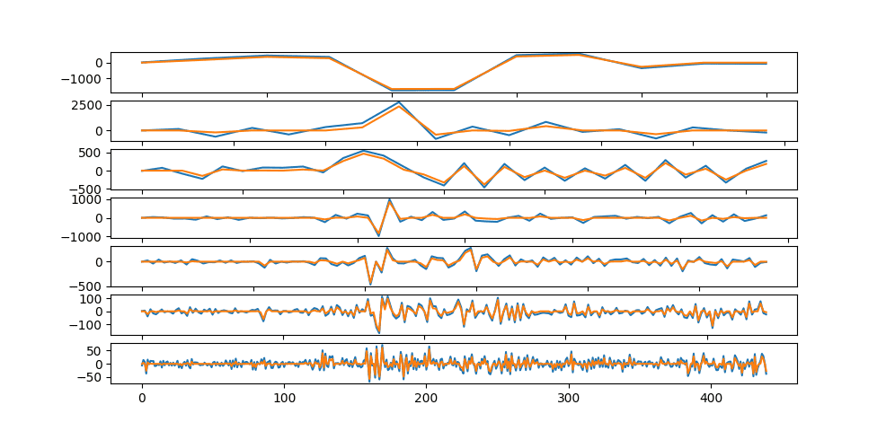
Synthesis of new series values using decompositions
As mentioned earlier, the result of the wavelet transform is a certain number of sequences ordered in time. These sequences, in turn, reflect the processes occurring inside the systems generating a series, decomposed over a certain frequency spectrum (Fig. 6), while the values of these sequences retain their order in time. Therefore, it is possible to analyze them as separate time series with subsequent modeling and prediction of new values in each frequency spectrum separately. At the same time, by synthesizing a series with new values, it is possible to obtain a forecast.
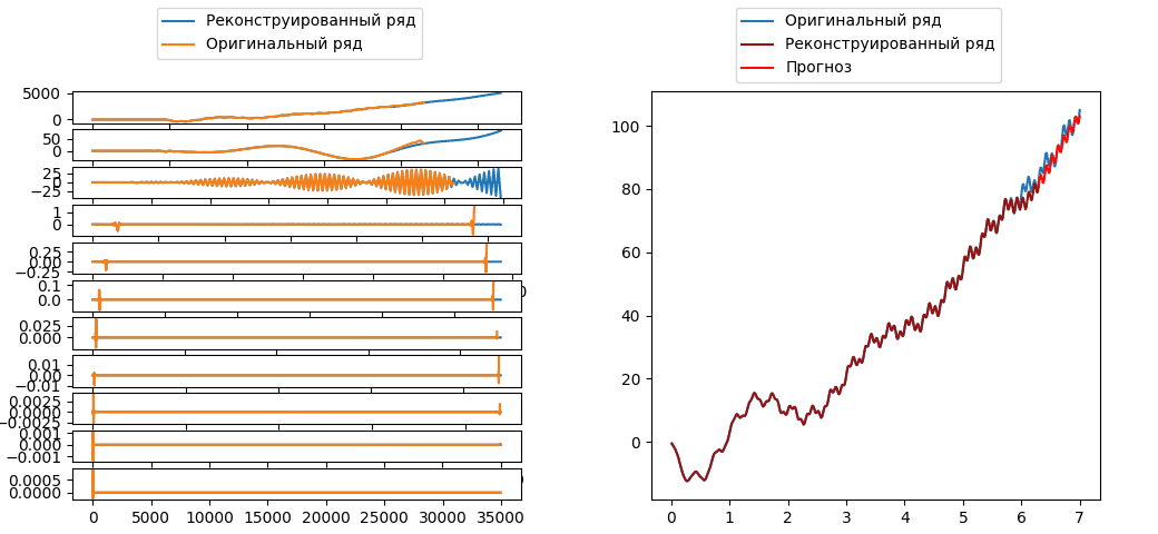
Let's say a sequence of numbers of length $N$ is received at the input of the discrete wavelet transform algorithm. One stage of such decomposition separates two components – low-frequency and high-frequency. These sets of values are also called approximation coefficients ($cA$) and detail coefficients ($cD$). Thus, if the length of the conversion filter equels L, then the length of the resulting sequences will be equal to:
$\displaystyle{ N_{cA}=N_{cD}-\left \lfloor \frac{N+L-1}{2} \right \rfloor }$
Сconsequently, in order to predict $\Delta$ the next values of the original series, it is necessary to generate $\DeltaN_{cA}=\DeltaN_{cD}$ new values of the desired sequences:
$\displaystyle{ \DeltaN_{cA}=\DeltaN_{cD}-\left \lfloor \frac{\Delta}{2} \right \rfloor }$
At the next stage, a set of approximation coefficients is already taken as the initial sequence and the algorithm is repeated. Therefore, if $i$ is the iteration number of the loop, then (7) and (8) follow:
$\displaystyle{ N_{i+1}=\DeltaN_{cA}_i=\left \lfloor \frac{N_{i+1}+L-1}{2} \right \rfloor }$
$\displaystyle{ \Delta_{i+1}=\DeltaN_{cA}_i=\left \lfloor \frac{\Delta_i}{2} \right \rfloor}$
Since time series represent some finite numerical sequences, their extrapolation becomes necessary during decomposition. This inevitably affects the data structure at the sequence boundaries [20], distorting the results to one degree or another. This effect has been well studied and is called the edge effect. In the classical application of wavelet analysis, this effect should only be borne in mind when working with a periodogram, there are many ways to extrapolate the signal [21] and the degree of confidence in such data is determined by the researcher. When restoring the original series, the effect is completely leveled. If this method is applied in the manner described in this section, the effect of this effect may affect the constructed model.
Let's say the following sequence acts as the initial series:
$\displaystyle{ y_i = y_1,y_2,...,y_n; n\inN }$
In this case, the results of the algorithm are sequences of coefficients:
$\displaystyle{ cA_i = cA_1, cA_2, ...cA_n_cA;n_{cA}\inN }$
$\displaystyle{ cD_i = cD_1, cD_2, ...cD_n_cD;n_{cD}\inN }$
Since in the calculation process the wavelet "slides" along the initial series, then with the length of the filter $L$, to calculate $cA_i$ and $cD_i$ following range of values is used $y$:
$\displaystyle{ \lbrack y_{i-\left \lfloor \frac{L}{2} \right \rfloor};y_{i+\left \lfloor \frac{L}{2} \right \rfloor}\rbrack }$
Therefore, edge effects occur at the boundaries of values within $\gamma=\lfloor\frac{L}{2}\rfloor$ elements from the edge.
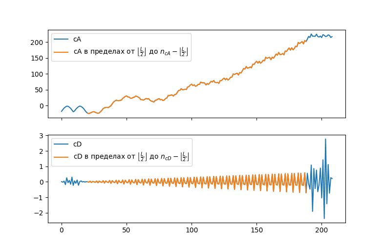
At the same time, the closer to the boundary, the more extrapolated values and the fewer real values of the series will be used in calculations. And therefore, the more powerful the influence of distorting factors will be. At the same time, the values of the series located within these limits carry useful information that will most strongly affect the data of points within the $\gamma$ values from the edge. Therefore, when building models, it is necessary to look for a compromise between two positions: the refusal to use values located within γ of the boundaries will mean the loss of data located at these points during the formation of the series model, at the same time, the use of these points will inevitably distort the results of the model.
Information context
Despite all their advantages, the problem with the above approaches is that they explore the time series as an exceptional abstraction, "in isolation from the outside world." This means that it is not possible to predict, for example, the position of a new bifurcation point in a series.
The usual practice in this case is to use the method of expert assessments. By analyzing the behavior of the system with the help of a certain pool of experts, it is possible to predict its behavior with a certain degree of probability. However, it should be borne in mind that in this case, the result obtained will contain a fair amount of subjectivity, which in one way or another may affect the accuracy of the forecast.
On the other hand, there are a huge number of Internet resources and platforms where various announcements, news and statements are published. There are cases when the statements of public speakers became the reasons for changes in the stock market. This can be called the information context of financial time series.
Having formed a training sample based on the price history of certain assets and their corresponding news posts, it is possible to try to train a model that predicts the behavior of the system.
By analogy with image generation algorithms [22], the input of such a model should include a certain set of numerical sequences representing a set of prices of an asset for a certain period, and a text prompt, which, in this case, is a set of news articles on a given asset, the primary analysis of which can be assigned to already existing ones in the open NLP model access. The token sets obtained in this way will, along with parameter sets, be input to the inner layers, the result of which will be some assessment of the semantic proximity of the data sets obtained at the input.
Thus, this algorithm should play the role of an expert in this field, assessing how the current parameters and appearance of the models correspond to the information context.
Conclusions
The study of time series requires, at its core, an integrated approach and the simultaneous application of various techniques that make it possible to identify one or another component of the time series. The considered methods of studying financial time series represent effective approaches to the analysis and modeling of dynamic processes. However, their main problem, like most others, is working with time series as abstractions, without taking into account the influence of external factors. This imposes certain requirements on the series itself, as well as certainly limits the predictive ability of the researcher. The expert assessment approach, although it is able to take into account the external information context, is vulnerable to cognitive distortions and subjective errors of the experts themselves.
Therefore, one of the promising areas for further research may be the integration of the information context into the analysis of financial time series. The introduction of news articles, announcements and statements as additional parameters of the analysis will allow us to take into account external factors that may affect the overall dynamics of the market. This will create more realistic and predictably valuable models that can take into account not only internal processes, but also market reactions to external events. In parallel, further research can and should be aimed at developing and improving existing methods for analyzing and modeling time series.
List of references
- Бизнес-прогнозирование: какой метод выбрать. / В. Клавдеева – Управление предприятием – 2023
- Теория статистики: Учебно-методический комплекс. / В.Г. Минашкин, Р.А. Шмойлова, Н.А. Садовникова, Л.Г. Моисейкина, Е.С. Рыбакова – М.: Изд. центр ЕАОИ. – 2008.
- Методы анализа и прогнозирования временных рядов / С. В.Поршнев, Н. Т.Сафиуллин – УрФУ - 2022
- Краткий курс теории случайных процессов. [Электронный курс] / М.К. Ризаева, Т.Ю Гаджиева - Дагестанский Государственный университет - 2018 - Режим доступа: [ссылка]
- Анализ времененных рядов. [Электронный ресурс] / А.Михайлов - 2023 - Режим доступа:[ссылка]
- Методы анализа временных рядов [Электронный ресурс] / Н.А. Хованова, И.А. Хованов - 2001 - Режим доступа:[ссылка]
- Анализ временных рядов и прогнозирование. / Н.А. Садовникова Р.А. Шмойлова – М.: «Футурис» – 2009
- Телятников З. Анализ временных рядов. / З.Телятников - k-tree - 2023
- Методы анализа временных рядов / Т.В. Саженкова, И.В. Пономарѐв, С.П. Пронь – Барнаул: Издво Алт. ун-та. – 2020
- Алгоритм поиска момента смены тренда во временных рядах метеорологических величин / А.Д. Кузнецов, А.Г. Саенко, О.С. Сероухова, Т.Е. Симакина - Вестник ТвГУ. Серия: Прикладная математика - 2019
- Спектрально-кореляционный анализ равномерных рядов / В.В. Витязев - Изд-во С.Петербю ун-та - 2001
- Understanding LSTM Network. [Электронный курс] / Б. Рохрер - 2015 - Режим доступа: [ссылка]
- Нейросети для работы с последовательностями / А. Янина - Учебник по машинному обучению - 2023
- Рекуррентные нейронные сети [Электронный курс] / В.Кустивкова - Приволжский научно-образовательный цент суперкомпьютерных технологий - 2018 - Режим доступа: [ссылка]
- Attention Is all you need. [Электронный курс] / A.Vaswani, N. Shazeer, N. Parmar, J. Uszkoreit, L. Jones, A. Gomez, L. Kaiser, I. Polosukhin - 2023 - Режим доступа: [ссылка]
- Оценка возможностей метода аналогов для текущего прогноза температуры воздуха / Восканян К.Л., Кузнецов А.Д., Сероухова О.С., Симакина Т.Е. - Вестник ТвГУ. - Серия: Прикладная математика. - 2019.
- Текущее прогнозирование экологических измерений на основе поиска аналогов / Восканян К.Л., Кузнецов А.Д., Сероухова О.С., Симакина Т.Е. - Сборник тезисов XI научно-прикладной международной конференции «Естественные и антропогенные аэрозоли» - 2018 г.
- Применение спектрального анализа при обработке геофмизческих данных / А.И. Банщиков, Б.А. Спасский - Вестник Пермского Университета - 2011
- PyWavelets: A Python package for wavelet analysis / Gregory R. Lee, Ralf Gommers, Filip Wasilewski, Kai Wohlfahrt, Aaron O’Leary – Journal of Open Source Software – 2019
- Анализ способов устранения краевого эффекта при спектральном анализе сигналов методом вейвлет-преобразования / Киселёв Б.Ю. – Международный журнал прикладных и фундаментальных исследований № 10 – 2017
- Statistics and Machine Learning Toolbox Documentatio [Электронный ресурс] / The MathWorks Inc. – 2023 – Режим доступа: [ссылка]
- Как работают нейронные генераторы картинок [Электронный ресурс] / А.Капранов - 2022 - Режим доступа: [ссылка]