The Hybrid Reciprocal Velocity Obstacle
Jamie Snape, Student Member, IEEE, Jur van den Berg, Stephen J. Guy, and Dinesh Manocha
Abstract—We present the hybrid reciprocal velocity obstacle for collision-free and oscillation-free navigation of multiple mobile robots or virtual agents. Each robot senses its surroundings and acts independently without central coordination or communication with other robots. Our approach uses both the current position and the velocity of other robots to compute their future trajectories in order to avoid collisions. Moreover, our approach is reciprocal and avoids oscillations by explicitly taking into account that the other robots also sense their surroundings and change their trajectories accordingly. We apply hybrid reciprocal velocity obstacles to iRobot Create mobile robots and demonstrate direct, collision-free, and oscillation-free navigation.
Index Terms—Collision avoidance, mobile robots, motion plan-ning, multirobot systems, navigation.
I. INTRODUCTION
Many recent works have considered the problem of navigating a robot in an environment composed of dynamic obstacles [1], [2], [3], [4], [5]. Some of the simplest approaches predict where the dynamic obstacles may be in the future by extrapolating their current velocities, and let the robot avoid collisions accordingly. However, such techniques are not sufficient when a robot encounters other robots, because treating the other robots as dynamic obstacles overlooks the reciprocity between robots. In other words, the other robots are not passive, but are actively trying to avoid collisions. Therefore, the future trajectories of other robots cannot be estimated by simply extrapolating their current velocities, since this would inherently cause undesirable oscillations in their trajectories [6].
In this paper, we present the hybrid reciprocal velocity obstacle for navigating multiple mobile robots or virtual agents which explicitly considers the reciprocity between robots. In-formally, reciprocity lets a robot take half of the responsibility for avoiding collisions with another robot and assumes that the other robot takes the other half. In a multirobot environment, this concept extends to every pair of robots. Each robot executes an independent feedback loop, in which it chooses its new velocity based on observations of the current positions and velocities of the other robots in close proximity. The robots do not communicate with each other, but implicitly assume that the other robots use the same navigation strategy based
on reciprocity. Our overall approach can also deal with both static and dynamic obstacles using a navigation roadmap.
The hybrid reciprocal velocity obstacle is an extension of the reciprocal velocity obstacle [6] that was introduced to address similar issues in multiagent simulation. However, the reciprocal velocity obstacle formulation has some limitations, particularly that it frequently causes agents to end up in a "reciprocal dance" [7] as they cannot reach agreement on which side to pass each other. To overcome this drawback, the hybrid reciprocal velocity obstacle enlarges the reciprocal velocity obstacle on the side that the robots should not pass by substituting the reciprocity velocity obstacle edge with the edge of a velocity obstacle [2]. Consequently, if a robot attempts to pass on the wrong side of another robot, then the robot has to give full priority to the other robot. If the robot chooses the correct side, then it can assume the cooperation of the other robot and retains equal priority.
We have implemented and applied our approach to a set of iRobot Create mobile robots moving in an indoor environment using centralized sensing from an overhead video camera and Bluetooth wireless remote control. Our experiments show that our approach achieves direct, collision-free, and oscillation-free navigation in an environment containing multiple mobile robots and dynamic obstacles even with some uncertainty in position and velocity. We also demonstrate the ability to handle static obstacles and the low computational requirements and scalability of the hybrid reciprocal velocity obstacle in two simulations of multiple virtual agents.
The rest of this paper is organized in the following manner. We begin by summarizing related prior work in Sec. II. We formally define the problem of navigating multiple mobile robots in Sec. III. In Sec. IV, we introduce our formulation of hybrid reciprocal velocity obstacles. In Sec. V, we use this formulation for navigating multiple mobile robots and take into account obstacles in the environment as well as uncertainty in radius, position, and velocity, and the dynamics and kinematics of the robots. We discuss implementation and present experimental results in Sec. VI.
II. PRIOR WORK
In this section, we give a brief overview of prior work on local and reactive navigation and existing variations of the velocity obstacle concept.
A. Local and Reactive Navigation
Reactive navigation differs from traditional global path planning approaches, for example [4], [8], [9], in that rather than planning complete paths to their goals, robots react only to their local environment at any moment in time.

Fig. 1. Construction of the hybrid reciprocal velocity obstacle (Sec. IV-C). (a) A configuration of two disc-shaped robots A and B in the plane with radii rA and rB, positions pA and pB, and velocities VA and VB, respectively. (b) The velocity obstacle VCA\B for robot A induced by robot B. (c) The reciprocal velocity obstacle RVCA \ B for robot A induced by robot B. (d) The hybrid reciprocal velocity obstacle HRVCA \ B for robot A induced by robot B. Note that VA is right of the centerline CL of RVCA\B, so the apex of HRVCA\B is the intersection point of the right side of RVCA\B and the left side of VCA\B.
Well-known reactive formulations include the dynamic window approach [3] and inevitable collision states [5], in addition to velocity obstacles [2]. Some approaches use a number of predefined discrete behaviors [10] or parameter space transformations [11]. Multiple robots may cooperate implicitly or by broadcasting their future intentions [12] or with limited bidirectional communication [13].
B. Collision Cones and Velocity Obstacles
A particularly successful concept for local and reactive navigation is the collision cone [1], especially in the form of a velocity obstacle [2], [14]. Velocity obstacles have been used in practice for applications such as warning drivers of impending highway collisions [15], navigating a robotic wheelchair through a crowded station [16], directing an autonomous robot within a pharmaceuticals plant [17], and mission planning for an unmanned aerial vehicle [18].
Several variations of velocity obstacles have been proposed for multirobot systems. Generally, these have attempted to incorporate the reactive behavior of the other robots in the environment. Formulations such as common velocity obstacles [19], recursive probabilistic velocity obstacles [20], [21], and reciprocal velocity obstacles [6] use various means to handle reciprocity, but all have shortcomings. Specifically, the common velocity obstacle and reciprocal velocity obstacle are limited to dealing with only two robots, while the recursive probabilistic velocity obstacle may fail to converge.
Approaches such as [22], [23], [24] truncate the collision cone to consider only collisions that will occur within a finite window of time.
III. PROBLEM DEFINITION
We consider the following formal definition of the problem of navigating multiple mobile robots.
Let there be a set of disc-shaped robots sharing an environment in the plane. The environment may also contain dynamic obstacles and static obstacles, which we assume can be identified by each robot as not actively adapting their velocity to avoid other robots. Each robot A has a fixed radius
r^, a current position p^, and a current velocity v^, all of which are known to the robot and may be measured by the other robots in the environment. Let each robot also have a goal located at pA^' and a preferred speed which are unknown to the other robots. The goal may simply be a fixed point chosen in the plane or the result of some external criteria, such as the output of a global planning or scheduling algorithm. The preferred speed is the speed that a robot would take in the absence of other robots or obstacles and may be similarly chosen manually or by some external algorithm. The robots may have dynamic and kinematic constraints.
The objective of each robot is to independently and simultaneously choose a new velocity at each time step to compute a trajectory toward its goal without collisions with any other robots or obstacles and with as few oscillations as possible. The robots should not communicate with each other or perform any sort of central coordination, but many assume that the other robots are using the same strategy to choose new velocities.
IV. VELOCITY OBSTACLES
In this section, we describe how robots avoid collisions with each other using velocity obstacles. We review the concepts of velocity obstacles and reciprocal velocity obstacles, and then introduce our formulation of hybrid reciprocal velocity obstacles that we use for navigating multiple mobile robots.
A. Velocity Obstacles
The velocity obstacle [2] was introduced for local collision avoidance and navigation of a robot amongst multiple moving obstacles. In two dimensions, it is defined as follows.

Fig. 2. A scenario where two robots select oscillating velocities as a result of using velocity obstacles (Sec. IV-A). (a) Robots A and B each choose the velocity closest to their current velocity that is outside the velocity obstacle induced by the other robot. (b) In the next time step, each robot has attained its new velocity, and since the new velocity leaves its previous velocity outside the velocity obstacle, it returns to that velocity in the following time step
Let A be a robot and let B be a dynamic obstacle moving in the plane. Let and pB denote the current positions of robot A and dynamic obstacle B, respectively, and let vB be the velocity of dynamic obstacle B, as shown in Fig. 1(a). It follows that the velocity obstacle for robot A induced by dynamic obstacle B, written VO4^, is the set of all velocities of robot A that will result in a collision between robot A and dynamic obstacle B at some future moment in time, assuming that dynamic obstacle B maintains a constant velocity v s.
More formally, let A e B = {a + b | a e A, b e B} be the Minkowski sum of robot A and dynamic obstacle B, and let -A = {-a | a e A} denote the robot A reflected in its reference point. Furthermore, let A(p, v) = {p + tv 11 > 0} be a ray starting at position p with direction v, then

A geometric interpretation of the region VC^s appears in Fig. 1(b). Note that the apex of the velocity obstacle is at v_e.
If robot A and dynamic obstacle B are both disc-shaped with radii r,4 and r_e, respectively, then the definition of the velocity obstacle (1) simplifies to

where D(p, r) is an open disc of radius r centered at p.
It follows that if robot A chooses a velocity inside VC>A\B, then robot A and dynamic obstacle B will potentially collide at some point in time. If the velocity chosen is outside VO4^, then a collision will not occur.
We note that the velocity obstacle is symmetric, is inside VO4^ if and only if vB is inside VC^, and translation invariant, is inside VO4^ (vB = v) if and only if + u is inside VCA\B (vB = v+u). By the convexity ofhalf-planes, the velocity obstacle is also convex, that is if v and u are in the left half-plane extending from the left edge of then (1 - t)v + tu is in the left half-plane extending from the left edge of VO4^ for all 0 < t < 1, and equivalently for the right half-plane extending from the right edge of .
The velocity obstacle has been successfully used to navigate one robot through an environment containing multiple dynamic obstacles by having the robot select a velocity in each time step that is outside any of the velocity obstacles induced by the dynamic obstacles [2], [16], [21]. Unfortunately, the velocity obstacle concept does not work well for navigating multiple robots where each robot is actively adapting its velocity to avoid the other robots since it assumes that other robots never change their velocities [19]. If all robots were to use velocity obstacles to choose a new velocity, there would inherently be oscillations in the trajectories of the robots [6]. More precisely, if robots A and B each select a new velocity outside the velocity obstacle of the other, then their old velocities are valid with respect to the velocity obstacle based on the new velocities. Hence, the robots oscillate back to the old velocities, as shown in Fig. 2.
B. Reciprocal Velocity Obstacles
The reciprocal velocity obstacle [6] addresses the problem of oscillations caused by the velocity obstacle by incorporating the reactive nature of the other robots. Instead of having to take all the responsibility for avoiding collisions, as with velocity obstacles, reciprocal velocity obstacles let a robot take just half of the responsibility for avoiding a collision, while assuming the other robot involved reciprocates by taking care of the other half.
More formally, when choosing a new velocity for robot A, the average is taken of its current velocity and a velocity outside the velocity obstacle induced by the other robot
B. It follows that the reciprocal velocity obstacle for robot A induced by B, written RVCA\B, is defined as

The geometric interpretation of RVCA\B in Fig. 1(c) illustrates that the velocity obstacle has been effectively translated such that its apex is at (v^ + vB )/2.
In theory, the reciprocal velocity obstacle formulation guarantees that if both robots A and B select a velocity outside the reciprocal velocity obstacle induced by the other, and both robots choose to pass each other on the same side, then the trajectories of both robots will be free of collisions and oscillations in the local time interval.
By the symmetry, translation invariance, and convexity of the velocity obstacle, it follows that if is in the left half-plane extending from the left edge of RVO4^ and vg^ is in the left half-plane extending from the left edge of RVO^ then v^f^ is in the left half-plane extending from the left edge of VO4^ (vB = vB^) and vg^ is in the left half-plane extending from the left edge of VC^(v^ = ). The equivalent statement holds for the right half-planes extending from the right edges of RVO4^ and RVC^. Hence there will not be collision if and are chosen, by the properties of the velocity obstacle [6].
The trajectories of the two robots can be shown to be free oscillations by the translation invariance of the velocity obstacle [6]. More formally, if v^f^ = w + u and = v - u, then w is inside RVC^ (vB = v, = w) if and only if w is inside RVO^ (vB = v + u, = w + u).
If each robot chooses the new velocity closest to the current velocity of the robot, then the robots will automatically pass each other on the same side [6], that is if = + u and = v B - u, then + u is outside RVO^ if and only if vB - u is outside RVC^.

Fig. 3. Two configurations of robots that cause robot A to be unable to select the velocity outside RVC>A\B closest to its current velocity VA, therefore increasing the possibility of reciprocal dances (Sec. IV-B). (a) The preferred velocity of robot A toward goal G is oriented in a different direction
to vA.(b) A third robot C causes the velocity outside RVC^\B closest to VA to be within RVCA\c, and so may potentially cause robot A to collide with robot C if taken.
Rather than choosing velocities closest to their current velocities, in order to make progress, robots A and B are typically required to select the velocity closest to their own preferred velocity , that is, the velocity directed from each robot towards its goal, as in Fig. 3(a). Furthermore, as shown in Fig. 3(b), the presence of a third robot C may cause at least one of the robots to choose a velocity even farther from its current velocity. Unfortunately, this means that robots may not necessarily choose the same side to pass, which may result in oscillations known as "reciprocal dances" [7].
While distinct from the oscillations caused by the velocity obstacle, reciprocal dances may be equally difficult for the robots to resolve and, in extreme circumstances, this behavior may become stable and the robots may oscillate forever. More precisely, there exists a configuration in which if is the closest velocity to which is outside RVO^ (vB = v, = w) and is the closest velocity to which is outside RVC^(vA = w, vB = v) then w is the closest velocity to which is outside RVO^ (vB = , = vAf^) andv is the closest velocity to which is outside
RVCB\A(vA = vAT, vB = vB^).
C. Hybrid Reciprocal Velocity Obstacles
To counter this situation, we introduce the hybrid reciprocal velocity obstacle, shown in Fig. 1(d). For robots A and B, if is to the right of the centerline of RVO^^, which implies by symmetry that vB is to the right of the centerline of RVO_B^, we wish robot A to choose a velocity to the right of RVO^. To encourage this, the reciprocal velocity obstacle is enlarged by replacing the edge on the side we do not wish the robots to pass, in this instance the left side, by the edge of the velocity obstacle VO4^. The apex of the resulting obstacle corresponds to the point of intersection between the right side of RVO^ and the left side of . If is to
the left of the centerline, we mirror the procedure, exchanging left and right. As a hybrid of a reciprocal velocity obstacle and a velocity obstacle, we call the result a hybrid reciprocal velocity obstacle, written ffRVO^.
The hybrid reciprocal velocity obstacle formulation has the consequence that if robot A attempts to pass on the wrong side of robot B, then it has to give full priority to robot B, as with the velocity obstacle. However, if it does choose the correct side, then it can assume the cooperation of robot B and retains equal priority, as for the reciprocal velocity obstacle. This greatly reduces the possibility of oscillations, while not
unduly over-constraining the motion of each robot. While it is still possible for the robots to pass on the wrong side of each other, this behavior is not stable because the robots may still pass on the correct side of each other in a future time step.
V. NAVIGATING MULTIPLE MOBILE ROBOTS
In this section, we show how we apply our hybrid reciprocal velocity obstacle formulation to navigating multiple mobile robots. We first describe the overall approach, and then explain how to take into account obstacles in the environment, uncertainty in radius, position, and velocity, and the dynamics and kinematics of the robots.
A. Overall Approach
Initially, in Sec. IV-C above, we have defined the hybrid reciprocal velocity obstacle for only two robots in an uncluttered environment. Suppose instead that we have a set of robots A sharing an environment with a set of dynamic and/or static obstacles O. Each robot Aj in A has a current position , velocity , and radius . Furthermore, each robot Aj has a preferred velocity

toward its goal centered at , where is the constant preferred speed of that robot.
The combined hybrid reciprocal velocity obstacle for robot Aj induced by all other robots and obstacles in the environment is the union of all hybrid reciprocal velocity obstacles induced by the other robots individually and all velocity obstacles generated by the obstacles, that is

This is illustrated in Fig. 4. The robot Aj should therefore select as its new velocity the velocity outside the combined hybrid reciprocal velocity obstacle that is closest to its preferred velocity:

We use the ClearPath efficient geometric algorithm [23] to compute this velocity. Following the ClearPath approach, which is applicable to many variations of velocity obstacles, we represent the combined hybrid reciprocal velocity obstacle as a union of line segments. The line segments are intersected pairwise and the intersection points inside the combined hybrid reciprocal velocity obstacle are discarded. The remaining intersection points, shown by white markers in Fig. 4 are permissible new velocities on the boundary of the combined hybrid reciprocal velocity obstacle. In addition we project the preferred velocity on to the line segments and also retain those points that are outside the combined hybrid reciprocal velocity obstacle, as indicated by the gray markers in Fig. 4.

Fig. 4. The combined hybrid reciprocal velocity obstacle for the dark-colored robot (Sec. V-A) is the union of all hybrid reciprocal velocity obstacles induced by the other robots individually. The intersection points of the line segments that are not inside the combined hybrid reciprocal velocity obstacle are indicated by white markers and the projections of the preferred velocity onto the line segments that are not inside the combined hybrid reciprocal velocity obstacle are indicated by gray markers. These points are the permissible new velocities computed by the ClearPath algorithm.
It is guaranteed that the velocity that is closest to the preferred velocity of the robot is in either of these two sets [23], and we choose that point as the new velocity for the robot.
If there are no permissible new velocities, we discard the hybrid reciprocal velocity obstacle of the farthest away robot or obstacle and repeat the ClearPath algorithm until a velocity outside the combined hybrid reciprocal velocity obstacle becomes available. It is possible that there may be collisions between robots, or deadlocks if they both stop, however we have only observed this issue on occasion in simulations with several hundred virtual agents.
While the robot should take the new velocity imme-diately, this may not be directly possible due to its kinematic constraints. Therefore, the velocity is transformed into a control input for the robot that will let the robot assume as soon as possible. We expand upon this transformation in Sec. V-E below.
The overall approach is summarized by the algorithm in Fig. 5. Note that we do not require the robots to communicate with each other. Robots use only the information that they can sense independently.
B. Obstacles
The presence of dynamic or static obstacles necessitates slight changes to our approach. In Sec. V-A above, the combined hybrid reciprocal velocity obstacle (2) uses velocity obstacles, rather than hybrid reciprocal velocity obstacles, for each obstacle in the environment since a robot cannot assume the cooperation of the obstacles to avoid collisions whichever side of the relevant reciprocal velocity obstacle the current velocity of the robot lies on. The velocity obstacle for a line static obstacle, constructed using the general definition (1) from Sec. IV-A above, is shown in Fig. 6.
An additional consideration is that an obstacle may block the path from the current position of a robot to its goal, hence causing the preferred velocity to be directed toward or through the obstacle. To account for this, we can incorporate a global navigation strategy, such as the probabilistic roadmap [8] or rapidly-exploring random trees [9], and use the nearest visible node of a covering roadmap as a waypoint or subgoal and direct the preferred velocity there rather than directly toward the ultimate goal. An example of part of such a roadmap is also illustrated in Fig. 6.

Fig. 6. The velocity obstacle for a line segment static obstacle O and part of a roadmap of subgoals to aid navigation to a goal G (Sec. V-B).
We have found the covering roadmap approach to be preferable to attempting to follow complete precomputed paths that are guaranteed not to collide with static obstacles since it
is unclear how to compute a preferred velocity that allows a robot to rejoin the path without oscillations if it has deviated from the path to avoid another robot or dynamic obstacle. Additionally, the precomputed path may not remain visible if the deviation of a robot from the path is large. When using a covering roadmap, a robot may simply choose another node, resulting in a different path to the goal.
C. Uncertainty in Radius, Position, and Velocity
To calculate the hybrid reciprocal velocity obstacles, each robot requires the radius, current position, and current velocity of every robot, and the position and physical extent of every obstacle. Because this data is obtained using sensors, it inevitably contains uncertainty. This may jeopardize the correct functioning of our approach.
We assume that each robot has onboard sensing and is able to measure the positions, or relative positions, of itself and every other robot or obstacle and that it has prior knowledge or is able to sense the radius of itself and the other robots. We use a Kalman filter [25], [26] to obtain accurate estimates of the radii, positions, and velocities of the robots and obstacles. In addition, the Kalman filter provides an estimate of the variance and covariance of the measured quantities.
If PA_ ~ N(p^4, ) is a bivariate Gaussian distribution of a measured position with mean and covariance T,PA, and PB ~ N(pB, Sj,^) is a bivariate Gaussian distribution of the measured position pB with mean pB and covariance Sj,^, then

is a bivariate Gaussian distribution of the measured relative position pB -with mean pB -pA and covariance ^PB_A. Moreover, if R^4 ~ N(rA,CTrA) is a Gaussian distribution of the measured radius r,4 and RB ~ N(rB ,o>_g) is a Gaussian distribution of the measured radius rB, then

is a Gaussian distribution of the measured r^4 + rB.
Assuming VB ~ N(vB, ) is a bivariate Gaussian distribution of the measured velocity vB, we use these distributions to construct the uncertainty-adjusted velocity obstacle, written VO>A^, as follows.
First, we expand the relative angle of the sides of the velocity obstacle cone to encompass the area corresponding to the Minkowski sum of the a disc of radius r A_+v,-^B and a linear transformation of a disc centered at pB - + v B by the covariance ^PB_A. Secondly, we move the sides of the velocity obstacle out perpendicularly by an amount large enough to encompass the linear transformation of a unit disc by the covariance . As the Gaussian distribution has infinitive extent, it is necessary to choose a finite segment of the distribution. In practice, we found one standard deviation around the mean to be acceptable, as shown in Fig. 7(a).
The uncertainty-adjusted reciprocal velocity obstacle RVO"A^, illustrated in Fig. 7(b), is constructed in a similar manner. We expand the relative angle of the sides of the reciprocal velocity obstacle cone to encompass the area corresponding to the Minkowski sum of the a disc of radius r ji+rB + o>^_g and a linear transformation of a disc centered at PB -pA+(VB +VB)/2 bythecovariance ^PB_A. Assuming that

is a bivariate Gaussian distribution of the measured (v,4 + vs)/2, where VA_ ~ N(VA, SVA) is a bivariate Gaussian distribution of the velocity vA, then we move the sides of the velocity obstacle out perpendicularly by an amount large enough to encompass the linear transformation of a unit disc by the covariance ^v^+B)/2. Note that if vA and vB are independent, then RVO>A^ will be comparatively smaller than VO*
V^A|B.
The uncertainty-adjusted hybrid reciprocal velocity obstacle HRVOA|B, shown in Fig. 7(c), is constructed from VO>A^ and RVc>A^ as explained in Sec. IV-C above. The combined uncertainty-adjusted hybrid reciprocal velocity obstacle HRVOA is constructed in an analogous way to the combined hybrid reciprocal velocity obstacle in Sec. V-A above. Any velocity obstacles VO^o for each obstacle O in the environment are expanded to uncertainty-adjusted velocity obstacles VO>A|Q as part of the construction.
D. Dynamic Constraints
Each robot is likely to be subject to dynamic constraints which reduce the velocities that it can attain within a time step At. Suppose robot A with current velocity v,4 has a maximum speed and maximum acceleration o"^, then the set of velocities from which to choose is reduced to

E. Kinematic Constraints
We can apply our approach to mobile robots with differential-drive constraints. Such robots, shown in Fig. 8, use a simple drive mechanism, that consists of two drive wheels mounted on a common axis with each wheel able to be independently driven in both forward and reverse directions.
The configuration of a differential-drive mobile robot is given by its position p = (x, y) and its orientation 6. If the wheel track of the robot is L, and the left and right wheel speeds are v and v,., respectively, then the configuration transition equations [27] are

Furthermore, the wheel speeds are bounded to a given maximum vmax, such that

The speeds of the wheels are the control input of the robot. When vl = v,, > 0, the robot will move straight forward, when vl > v,, > 0, it will arc right, and when vl = -v,, = 0, it will spin in place. The center of the robot is able to follow any continuous path within the environment [27].

Fig. 7. Construction of the uncertainty-adjusted hybrid reciprocal velocity obstacle (Sec. V-C). (a) The uncertainty-adjusted velocity obstacle VO>A|B takes into account uncertainty in the radii rA and r_e, positions VA and vB, and the velocity vB. Recall that the velocity VA is not used in the construction of a velocity obstacle. (b) The uncertainty-adjusted reciprocal velocity obstacle RVOA|B additionally takes into account uncertainty in the velocity VA. (c) The uncertainty-adjusted hybrid reciprocal velocity obstacle HRVO>A|B. Since v^A is right of the centerline CL* of RVOA|B, the apex of HRVO>A|B is the intersection point of the right side of RVOAB and the left side of VO*A\B.

Fig. 8. The kinematics of a differential-drive mobile robot (Sec. V-E). Each wheel is attached to a separate motor and may take a different speed. Note that the robot can spin in place and follow any continuous path.
As indicated in Sec. V-A, we must transform the velocity from (3) to wheel speeds v and vr, given the current orientation 6 of the robot. We choose to set v and vr such that is obtained after a prescribed amount of time T to ensure smooth motion. More formally, suppose that = (v^, ). Then, the target orientation is 6' = tan^^(v^ /v^) and the target speed is ||vA^|^. The difference between the target orientation and current orientation is A6 = 6' - 6, such that A9 G [-n, n]. To move from the current orientation 9 to the target orientation 6' in T time, it follows directly from (6) that

To obtain the target speed, it follows from (4) and (5) that

The desired values of v and v,, may be calculated from the system of equations formed by (8) and (9).
If the constraints of (7) invalidate the computed values of v and v,,, we first attempt to move v and vr into the interval [-vmax,vmax] while keeping vr - v constant, such that the
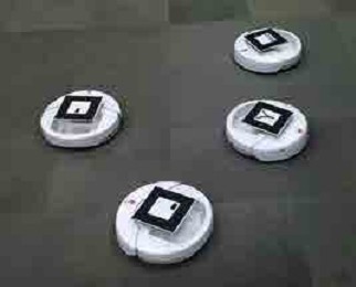
Fig. 9. Four iRobot Create mobile robots in our experimentation setting (Sec. VI-A). Note the fiducial attached to the top of each robot to allow it to be tracked by an overhead video camera.
target orientation is obtained after T time. If, after this, v and v,, still do not satisfy the constraints of (7), in which case |vr- - v | > 2v"^, then v and vr are clamped to the extremes of the interval, such that the robot maximally rotates in place.
The choice of T must be small enough to allow the robot to react quickly to other robots and obstacles in its path. However, if set lower than the duration At of each time step, the robot will overshoot its target orientation, leading to oscillations in its trajectory. A low value of T may also result in less smooth paths, since the robot may have to frequently rotate in place to achieve its target orientation. In practice, we have found that a value of T = 3At yields good results.
VI. EXPERIMENTATION
In this section, we describe the implementation of our approach and report results from our experiments involving multiple mobile robots.
A. Implementation Details
We implemented our approach for a set of iRobot Create mobile robots using centralized sensing and wireless remote control.
The iRobot Create is a differential-drive mobile robot, based on the iRobot Roomba vacuum-cleaning robot [28]. It has two individually actuated wheels and a third passive caster wheel for balance. The maximum speed of the robot is 0.5m/s in both forward and reverse directions, its shape is circular with radius 0.17 m, and it has a mass of less than 2.5 kg. The limited sensing power of the iRobot Create does not allow it to localize itself with any degree of accuracy.
For convenience, the robots were tracked centrally using fiducials, Fig. 9, within a 6rr^ indoor space using an overhead video camera connected to a desktop computer. Images were captured at a resolution of 1024x768 and refresh rate of 30Hz, and were processed using the ARToolKit augmented reality library [29] to determine the position and orientation of each robot, with an absolute error of less than 0.01 m. The velocity of each robot was inferred from the position and orientation measurements using a Kalman filter.
All calculations were performed on a 2.53 GHz Intel Core 2 Duo system with 8GiB of memory running Microsoft Windows 7. However, to ensure that our approach applies when each robot uses its own on-board sensing and computing, only the localization was carried out centrally. The other calculations for each robot were performed in separate and independent processes that did not communicate with each other. The computed wheel speeds, encoded in 4b serial data packets, were sent to the robots over a Bluetooth virtual serial connection at a speed of 57.6kb/s and average latency of 0.5 s.
B. Experimental Results
Using the iRobot Create mobile robots, we tested our approach in the following two scenarios:
1) Five robots are spaced evenly on the perimeter of a circle. Their goal is to navigate to the antipodal position on the circle. The robots will meet and have to negotiate around each other in the center (Fig. 10).
2) One robot takes the role of a dynamic obstacle, moving at a constant velocity. The other robots have to cross its path to navigate to their goals (Fig. 11).
In addition, we tested the ability to handle to handle static obstacles and the scalability of our approach in two simulated scenarios:
3) Four virtual agents must navigate from one side of a rectangle to the other, negotiating around each other in the center. Blocking their path are two static obstacles which form a passage through which they must pass
(Fig. 12).
4) One hundred virtual agents are spaced evenly on the perimeter of a circle. Their goal is to navigate to the antipodal position on the circle. The agents will meet and have to negotiate around each other in the center
(Fig. 13).
Fig. 10 shows traces of the five robots in Scenario 1 for three variations of the velocity obstacle formation. In Fig. 10(a),
when the robots use velocity obstacles, the traces are not smooth due to oscillations, while in Fig. 10(b), for reciprocal velocity obstacles, the beginnings of the traces are not smooth due to reciprocal dances. The traces in Fig. 10(c), with robots navigating using hybrid reciprocal velocity obstacles, show no oscillations or reciprocal dances over their entire lengths for any robot. In each experiment, the velocities of the robots were updated at a rate of 30 Hz, limited by the refresh rate of the tracking camera.
Scenario 2 in Fig. 11 shows that the hybrid reciprocal velocity obstacle formulation can naturally deal with the presence of a dynamic obstacle that may not necessarily adapt its motion to the presence of other robots. Two robots increase speed to cross ahead of the dynamic obstacle, while the third slows and crosses behind. As described in Sec. V-A and Sec. V-B above, the combined hybrid reciprocal velocity obstacle for each robot is the union of the hybrid reciprocal velocity obstacles of the other two robots and the velocity obstacle of the dynamic obstacle. Note that we do not consider how to identify between a robot and a dynamic obstacle, simply that our formulation is capable of handling the distinction should it be made.
Scenario 3 in Fig. 12 shows traces from our simulation of four virtual agents navigating though a passage while avoiding collisions with the static obstacles and each other. The agents merge into two lines before the passage and pass through in double file. Once they have negotiated the passage, they move towards their goals.
Fig. 13 shows three screenshots of Scenario 4, our simulation with one hundred virtual agents. Fig. 13(a) shows the starting configuration, Fig. 13(b) shows the agents approaching the center of the circle, and Fig. 13(c) shows the agents moving towards the perimeter of the circle having passed the center. All computations were completed in less than 15 per agent per time step on one core. The timing of Scenario 4 for three variations of velocity obstacles is shown in Table I. Given the reactive nature of the hybrid reciprocal velocity obstacle formulation, it is difficult to calculate any formal bound on the computation time.
Table II and Fig. 14 show the timing for Scenario 4 with an increasing number of virtual agents moving across a circle with a circumference that has been increased proportionally to the number of agents. This shows that our formulation can navigate up to one thousand virtual agents before the computation time per time step exceeds the 30Hz refresh rate of a sensor such as the tracking camera used in our experiments with iRobot Create mobile robots.
Table III and Fig. 15 show the collisions in Scenario 4 with an increasing number of virtual agents moving across a circle with a fixed circumference so that the density of agents is increased and free space reduced. As the number of virtual agents exceeds one hundred, a small, but increasing, number of collisions per time step are observed, as there is insufficient space left uncovered by hybrid reciprocal velocities for some agents.
Videos of these scenarios are available online at http://gamma.cs.unc.edu/HRVO/.

Fig. 10. Traces of five robots moving simultaneously across a circle (Scenario 1 in Sec. VI-B) using (a) velocity obstacles, (b) reciprocal velocity obstacles, and (c) hybrid reciprocal velocity obstacles.

Fig. 11. Traces of three robots moving simultaneously across the path of a single dynamic obstacle (Scenario 2 in Sec. VI-B) using hybrid reciprocal velocity obstacles. The trace corresponding to the dynamic obstacle is the near-horizontal line.

Fig. 12. Traces of four virtual agents moving simultaneously across a rect-angle, passing through a passage formed by two static obstacles (Scenario 3 in Sec. VI-B) using hybrid reciprocal velocity obstacles.
TABLE I
TIMING OF SIMULATIONS OF ONE HUNDRED VIRTUAL AGENTS MOVING SIMULTANEOUSLY ACROSS A CIRCLE (SCENARIO 4 IN SEC. VI-B) USING VELOCITY OBSTACLES, RECIPROCAL VELOCITY OBSTACLES, AND HYBRID RECIPROCAL VELOCITY OBSTACLES.

TABLE II
TIMING OF SIMULATIONS OF INCREASING NUMBERS OF VIRTUAL AGENTS MOVING SIMULTANEOUSLY ACROSS A CIRCLE OF INCREASING CIRCUMFERENCE USING HYBRID RECIPROCAL VELOCITY OBSTACLES.

TABLE III
COLLISIONS IN SIMULATIONS OF INCREASING NUMBERS OF VIRTUAL
AGENTS MOVING SIMULTANEOUSLY ACROSS A CIRCLE OF FIXED
CIRCUMFERENCE USING HYBRID RECIPROCAL VELOCITY OBSTACLES.

VII. CONCLUSION, LIMITATIONS, AND FUTURE WORK
In this paper, we have introduced the hybrid reciprocal velocity obstacles for navigating multiple mobile robots or virtual agents sharing an environment. We take into account obstacles in the environment, uncertainty in radius, position, and velocity. We also consider the dynamics and kinematics of the robots, allowing us to implement our approach on iRobot Create mobile robots. Our formulation explicitly considers reciprocity, such that each robot can assume that other robots are cooperating to avoid collisions, but each of the robots acts completely independently without central coordination, and does not communicate with other robots. We show direct, collision-free, and oscillation-free navigation.
In future, we would like to develop a more sophisticated and less conservative model of uncertainty, that takes into

Fig. 13. Screenshots of one thousand virtual agents moving simultaneously across a circle (Scenario 4 in Sec. VI-B) using hybrid reciprocal velocity obstacles.

Fig. 14. Plot of the timing of simulations of increasing numbers of virtual agents moving simultaneously across a circle of increasing circumference using hybrid reciprocal velocity obstacles (Table II in Sec. VI-B).

Fig. 15. Plot of the collisions in simulations of increasing numbers of virtual agents moving simultaneously across a circle of fixed circumference using hybrid reciprocal velocity obstacles (Table III in Sec. VI-B).
account more than simply uncertainty in position and velocity originating from the sensors of the robot, and apply it to the hybrid reciprocal velocity formulation.
Each of the robots currently receives their sensor readings from an overhead video camera. As a next step, we would like to equip each robot with purely localized sensing and comput-
ing, as in [30], which uses odometry, orientation sensors, and relative positions to estimate global positions. Our approach can be applied without adaptation if data is gathered locally, and the hybrid reciprocal velocity obstacles are defined just as well using only the relative positions and velocities of the robots.
At present, we assume in general that a velocity outside all hybrid reciprocal velocity obstacles exists. We would also like to relax this assumption to accommodate very dense scenarios without observing any collisions or deadlocks when the space is entirely covered by hybrid reciprocal velocity obstacles. Also, our method for incorporating static obstacles does not allow for navigation through some narrow passages for similar reasons.
Our current implementation considers only differential-drive constraints, but we would like to adapt our approach for other kinematic systems, in particular car-like robots as they have similar kinematic constraints [27]. We would also like to be able to handle more complex dynamic constraints.
REFERENCES
- A. Chakravarthy and D. Ghose, "Obstacle avoidance in a dynamic en-vironment: A collision cone approach," IEEE Trans. Syst. Man Cybern. A-Syst. Hum., vol. 28, no. 5, pp. 562-574, Sep. 1998.
- P. Fiorini and Z. Shiller, "Motion planning in dynamic environments using velocity obstacles," Int. J. Robot. Res., vol. 17, no. 7, pp. 760-772, Jul. 1998.
- D. Fox, W. Burgard, and S. Thrun, "The dynamic window approach to collision avoidance," IEEE Robot. Autom. Mag., vol. 4, no. 1, pp. 23-33, Mar. 1997.
- D. Hsu, R. Kindel, J.-C. Latombe, and S. Rock, "Randomized kinodynamic motion planning with moving obstacles," Int. J. Robot. Res.,vol. 21, no. 3, pp. 233-255, Mar. 2002.
- S. Petti and T. Fraichard, "Safe motion planning in dynamic environments," in Proc. IEEE RSJ Int. Conf. Intell. Robot. Syst., Edmonton, AB, Canada, Aug. 2005, pp. 2210-2215.
- J. van den Berg, M. Lin, and D. Manocha, "Reciprocal velocity obstacles for real-time multi-agent navigation," in Proc. IEEE Int. Conf. Robot. Autom., Pasadena, CA, May 2008, pp. 1928-1935.
- F. Feurtey, "Simulating the collision avoidance behavior of pedestrians," Master's thesis, Dept. Elect. Eng., Univ. Tokyo, Tokyo, Japan, 2000.
- L. E. Kavraki, P. Svestka, J.-C. Latombe, and M. H. Overmars, "Probabilistic roadmaps for path planning in high-dimensional configuration spaces," IEEE Trans. Robot. Autom., vol. 12, no. 4, pp. 566-580, Aug.1996.
- J. J. Kuffner, Jr. and S. M. LaValle, "RRT-connect: An efficient approach to single-query path planning," in Proc. IEEE Int. Conf. Robot. Autom., vol. 2, San Francisco, CA, Apr. 2000, pp. 995-1001.
- L. Pallottino, V. G. Scordio, A. Bicchi, and E. Frazzoli, "Decentralized cooperative policy for conflict resolution in multivehicle systems," IEEE Trans. Robot., vol. 23, no. 6, pp. 1170-1183, Dec. 2007.
- J.-L. Blanco, J. Gonzalez, and J.-A. Fernandez-Madrigal, "Extending obstacle avoidance methods through multiple parameter-space transfor-mations," Auton. Robot., vol. 24, no. 1, pp. 29^8, Jan. 2008.
- S. Pedduri, K. M. Krishna, and H. Hexmoor, "Cooperative navigation function based navigation of multiple mobile robots," in Proc. Int. Conf. Integr. Knowl. Intensive Multi-Agent Syst., Waltham, MA, Apr.-May 2007, pp. 277-282.
- K. E. Bekris, K. I. Tsianos, and L. E. Kavraki, "A decentralized planner that guarantees the safety of communicating vehicles with complex dynamics that replan online," in Proc. IEEE RSJ Int. Conf. Intell. Robot. Syst., San Diego, CA, Oct.-Nov. 2007, pp. 3784-3790.
- F. Large, S. Sckhavat, Z. Shiller, and C. Laugier, "Using non-linear velocity obstacles to plan motions in a dynamic environment," in Proc. IEEE Int. Conf. Contr. Autom. Robot. Vis., vol. 2, Singapore, Dec. 2002, pp. 734-739.
- Z. Shiller, R. Prasanna, and J. Salinger, "A unified approach to forward and lane-change collision warning for driver assistance and situational awareness," in Intelligent Vehicle Initiative (IVI) Technology Controls and Navigation Systems. Warrendale, PA: SAE International, Apr. 2008, paper 2008-01-0204.
- E. Prassler, J. Scholz, and P. Fiorini, "Navigating a robotic wheelchair in a railway station during rush hour," Int. J. Robot. Res., vol. 18, no. 7, pp. 711-727, Jul. 1999.
- P. Fiorini and D. Botturi, "Introducing service robotics to the pharmaceutical industry," Intell. Serv. Robot., vol. 1, no. 4, pp. 267-280, Oct. 2008.
- J. S. Dittrich, F. Adolf, A. Langer, and F. Thielecke, "Mission planning for low-flying unmanned rotorcraft in uncertain environments," presented at AHS Int. Spec. Mtg. Unmanned Rotorcraft, Chandler, AZ, Jan. 2007.
- Y. Abe and M. Yoshiki, "Collision avoidance method for multiple autonomous mobile agents by implicit cooperation," in Proc. IEEE RSJ Int. Conf. Intell. Robot. Syst., vol. 3, Maui, HI, Oct.-Nov. 2001, pp. 1207-1212.
- B. Kluge and E. Prassler, "Recursive probabilistic velocity obstacles for reflective navigation," in Field and Service Robotics: Recent Advances in Research and Applications, ser. Springer Tracts in Advanced Robotics, S. Yuta, H. Asama, S. Thrun, E. Prassler, and T. Tsubouchi, Eds. Berlin, Germany: Springer, Jul. 2006, vol. 24, pp. 71-79.
- C. Fulgenzi, A. Spalanzani, and C. Laugier, "Dynamic obstacle avoidance in uncertain environment combining PVOs and occupancy grid," in Proc. IEEE Int. Conf. Robot. Autom., Rome, Italy, Apr. 2007, pp. 1610-1616.
- O. Gal, Z. Shiller, and E. Rimon, "Efficient and safe on-line motion planning in dynamic environments," in Proc. IEEE Int. Conf. Robot. Autom., Kobe, Japan, May 2009, pp. 88-93.
- S. J. Guy, J. Chhugani, C. Kim, N. Satish, M. Lin, D. Manocha, and P. Dubey, "ClearPath: Highly parallel collision avoidance for multi-agent simulation," in Proc. ACM SIGGRAPH Eurographics Symp. Comput. Animat., New Orleans, LA, Aug. 2009, pp. 177-187.
- J. van den Berg, S. J. Guy, M. Lin, and D. Manocha, "Reciprocal n-body collision avoidance," in Proc. Int. Symp. Robot. Res., Lucerne, Switzerland, Aug.-Sep. 2009.
- R. E. Kalman, "A new approach to linear filtering and prediction problems," Trans. ASME-J. Basic Eng., vol. 82, pp. 35-45, Mar. 1960.
- G. Welch and G. Bishop, "An introduction to the Kalman filter," Dept. Comput. Sci., Univ. N. Carolina Chapel Hill, Chapel Hill, NC, Tech.Rep. 95-041, 1995, revised Jul. 2006.
- S. M. LaValle, Planning Algorithms. Cambridge, U.K.: Cambridge Univ. Pr., May 2006, ch. 13, pp. 590-650.
- J. L. Jones, N. E. Mack, D. M. Nugent, and P. E. Sandin, "Autonomous floor-cleaning robot," U.S. Patent 6 883 201, Apr. 26, 2005.
- H. Kato and M. Billinghurst, "Marker tracking and HMD calibration for a video-based augmented reality conferencing system," in Proc. IEEE ACMInt. WorkshopAugment. Real., San Francisco, CA, Oct. 1999, pp. 85-94.
- S. I. Roumeliotis and I. M. Rekleitis, "Propagation of uncertainty in cooperative multirobot localization: Analysis and experimental results,"Auton. Robot., vol. 17, no. 1, pp. 41-54, Jul. 2004.