
Baenko Dmitry
Mining faculty
Department of development of mineral deposits
Specialty Development of mineral deposits
Mathematical modeling of the deformation of the rock mass at different values of laying hard protective structures
Supervisor: Doctor of Technical Sciences, Professor Podkopaev Sergey
Abstract
Contents
- Introduction
- Relevance of the topic
- 1. Selecting a method of mathematical modeling
- 2. Statement of the problem of modeling
- 3. Creating a mathematical model
- Conclusions
- References
Introduction.
Before conduct comprehensive laboratory studies necessary to carry out mathematical modeling to establish the possibility of using the proposed technology and the mechanism of squeezing out bedrock security structures of various designs.
In practice calculations using both analytical [ 1 ], and numerical methods [ 2 ]. The first is based on the mathematical methods for solving boundary value problems, usually complex and labor ¬ doemkih and quite often limited by simple geometric shapes of bodies and loading schemes. Numerical methods, which include, in particular, finite difference method, the method of boundary integral equations, boundary element method, finite element method and other methods, in contrast, are not limited to any form of bodies, nor FPIC ¬ bong load application. This, along with the omnipresence of powerful computational techniques you contributes to the diffusion of the engineering environment.
Computational methods:
- finite difference method
- discrete element method
- boundary element method
- Finite Element Method
Finite Element Method (FEM) is currently the standard for solving problems of solid mechanics by means of numerical algorithms.
Actuality.
Once popular method of finite differences, and the claim to universality boundary element method (boundary integral equations) now occupy fairly narrow niche, limited research or special tasks. FEM took the leading position with the ability to simulate a wide range of objects and phenomena. The vast majority of the structural elements, components and structures made of various materials having different natures, can be calculated by the FEM. At the same time, of course, you need to consider inevitable in any numerical approximation of the conventions and error. Therefore, the question of correspondence between the calculated model and reality is perhaps the main using analysis software. Despite the fact that such programs are more or less detailed documentation, they are still to some extent a black box. This means a certain unpredictability of the results, as well as some arbitrariness in their interpretation. Consequently, the quality of the findings made on the basis of results depends entirely on the skill, as well as in relation to the calculation of strength, a fundamental familiarity with the basics of FEM.
Numerical same methods are used to solve complex problems, each of which is almost unique in its boundary conditions, fluid properties. The results of such solutions for a wide range of users are of interest mainly as illustrative ¬ tion efficiency method of solution and to a lesser extent by themselves. Discrete element methods require processor-intensive computer; this limits the length of the model or the number of particles. The finite element method provides an opportunity to take into account in the calculation of different ¬ shaped and complex properties of soils, rather than two indices (E and v or C and φ). FEM thereby stimulated the development of test methods of soils and rocks, and new theories of strength and deformability.
Also, the benefits of FEM include the possibility of reducing the problem to a system of linear or nonlinear algebraic equations directly, without pre-formulation of their differential counterparts. Furthermore the finite element method has attracted the attention of researchers mainly the property that the continuum is broken down into a number of elements that can be considered as a specific part of it. Basic procedures FEM standard and do not depend on the dimension and the type of finite element, which allows for the unification of these procedures and to create software for the calculation of structures and a broad class of applications.
1. Selecting a method of mathematical modeling
Finite element method combined with powerful computer models allow the use of materials of almost any complexity. Thanks FEM have a real opportunity to move to the calculation not only concrete, but concrete structures under complex stress state. Reinforced concrete, as is known, is a complex material consisting of concrete and steel reinforcement working together, but with different mechanical properties. FEM applied to the calculation of reinforced concrete structures is not only a numerical analysis method, but also serves as a simulation tool, when the material model reflects the specificity of the finite element method.
The method FEM discretization object is to solve the equations of continuum mechanics under the assumption that these relations are carried out within each of the elementary regions. These areas are called finite elements. They may correspond to the real part of the space, such as spacing elements, or be a mathematical abstraction elements as bars, beams, plates or shells.
Within Finite element assigned properties, limited to an object area (this can be, for example, the characteristics of rigidity and strength of the material, density, etc.) and describes the values of the field of interest (as applied to the mechanics of this displacement, deformation, pressure, etc.). Parameters in the second group are assigned to the nodes of the element, and then introduced interpolate functions by which the respective values can be calculated at any point within the element or on its boundary. Mathematical description of the problem boils down to the element to tie in knots acting factors. In continuum mechanics, as a rule, travel and effort.
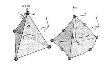
Figure 1 - Three-dimensional finite elements
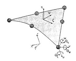
Figure 2 - Parabolic finite element surface

Figure 3 - Finite elements beams and bar
Algorithm application MKE following:
1. Performed sampling volume occupied part or assembly to the elements, or, as they say, the finite element mesh is constructed. To surround the body region is partitioned into tetrahedra with faces approximated by linear (linear dependence on the coordinates) or parabolic functions of the coordinates. For surface models - on flat (linear) or curved (parabolic dependence) triangles;
2. Finite elements for spatial degrees of freedom are moving in the direction of the axes of the local coordinate system of the element. For end shells to three elements in each node movements are added by three angles of rotation normal to the middle surface region of the approximated element relative to the same axes;
3. Determined according to convert displacements and rotation angles of the nodes to the global coordinate system;
4. Calculated stiffness matrix of finite elements. In the formula for calculating the components of the finite element stiffness matrices addition to the coordinates of nodes includes the elastic moduli and Poisson's ratios of materials. That is, if the assembly is analyzed, then, depending on the details of membership of an element in calculating the stiffness matrices of elements using the appropriate characteristics of the material stiffness;
5. The resulting stiffness matrix using the transition from dependency to local coordinate systems are transformed into global element in the global coordinate system;
6. Stiffness matrix presented in the global coordinates, the union ¬ nyayutsya the global stiffness matrix [ K ];
7. The user-boundary conditions, static and kinematic given to the loads and displacements at the nodes, expressed in the global coordinate system, and are included in the column of effort [ F ];
8. The resulting linear system of equations of the form [ K ] * [ A ] = [ F ] is solved for column movements. This is the most time-consuming step of the calculation. Solutions are used for iterative or direct methods. The stiffness matrix, is typically stored in a compact form, the structure of which is determined before the filling stage of its stiffness matrices of elements;
9. For each finite element, with displacement (rotation angles) at the nodes and the approximating functions are calculated deformation. If linear elements - deformation within the constant elements, if the elements of parabolic - strain vary linearly. On the basis of the voltage computed in the deformation elements. If necessary (software feature) voltage at the nodes of adjacent elements are averaged (this is also a very important stage, are solved differently in different programs), followed by recalculation of stress within each element;
10. Based on the components of the stress-strain state and strength parameters of the material (s), the computation of equivalent stress on any strength criterion.
Quite often modules nonlinear analysis of FEM programs are a superstructure on the base part, responsible for the elastic structural analysis.
Nonlinear problems are characterized by a nonlinear relationship between the operating factors and the response of the system to them. In addition, often the boundary conditions (applied load and displacement) change over time. To account for this phenomenon introduces the concept of time curve. Its meaning is that the input parameter having the dimension of time, and depending on its value, it defines the conditions are assigned. That is actually constructed diagrams in which the abscissa - this time, and the ordinate is power, power, movement, etc. If calculated to contain material, the characteristics of which may be time dependent, the parameter corresponds to the physical time. Otherwise, it is an abstract value, the scope of which is chosen for reasons of convenience representation of curves. In most applications, there are three methods used for different classes of problems.
2 Statement of the problem of modeling
There are many ways of protecting the mines, one of the most effective ways - the construction of the cast strip hardening compositions after stope
Essence of the method: after passing complex purification and extraction of minerals (Figure 4a), erected formwork (Figure 4b), which is placed inside the quick-mix concrete (Figure 4c).
Based on practices used in the construction of buildings - in the presence of soft soil at the base of the foundation to enhance its stability performance inception of the foundation. Decision was made using the software package PLAXIS 2D - working with the finite element method, to test the impact uglubki security structures relative soil, the state generation, as well as to determine the optimal amount of penetration. In PLAXIS 2D software package was created five models of rock mass. One model with standard layout cast strip + four models with varying degrees of penetration of security structures.
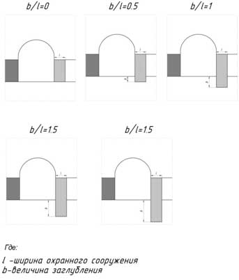
Figure 4 - Diagram deepening security structures
3 Creating a mathematical model
After starting the program, a dialog box Create / Open project (Figure 5), where you can open an existing or create a new project.
After selecting "New Project" window appears General settings (General Options), consisting of two tabs Project (Project) and Dimensions (Dimensions) (Figs. 6 and 7).
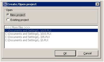
Figure 5 - Dialog Box Create / Open project
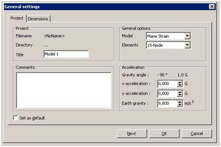
Figure 6 - Project tab window General settings
General Options. The first stage of each task is to set the basic parameters of the finite element model. This is done in the General settings (General Options). These settings include the description of the task, the type of calculation, the basic element type, the basic units and the size of the drawing field. To enter the relevant parameters for the calculation of the foundation, do the following:
In the Title (Name) tab Project (Project), we write the name of the «Model 1»
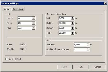
Figure 7 - Dimensions tab window General settings
In the General Type of task (Model) and the type of basic elements (Elements). In the combo box, select Model Plane Strain, and in the Elements - 15-noded (15 angled triangular element).
Under Acceleration (acceleration) indicates the value specified angle gravity equal to -90 º and extending in the vertical direction (down). Apart from the normal gravity values for psevdodinamicheskih calculations can be administered independent of each other acceleration components. Clicking () located beneath the tabs go to the tab Dimensions (Dimensions).
In the Units (Units) tab Dimensions (Dimensions) leave the default units:
- Length (L) - m (m);
- Force (load) - kN (kN);
- Time (time) - night (day)).
In the Geometry dimensions (geometry) introduced the planned size of the drawing field.
In the Grid (Grid) is defined grid. With the help of a grid on the screen displays a matrix of dots, which can be taken as a starting point. It can also be used for instant reference to the regular points during the creation of a geometric model. The distance between points is determined by the value given in the Spacing (Pitch). The distance between the anchor points may be further divided into smaller intervals by setting field Number of intervals the number of intervals
To confirm settings will click .
After completing the general parameters, appears a drafting field with the origin and the direction of the coordinate axes. The X-axis directed to the right, and the axis Y - up. Geometric model can be created anywhere, but within the size of the drawing field. Geometry line - to create objects - (geometric line) is already active. This option can also be selected from the first row of buttons on the toolbar that contains the geometric objects, or from the menu Geometry. With the tool Geometry line traceable region further modeling - By using Plaxis is defined cluster.
Boundary conditions. Boundary conditions can be selected from the second row of the toolbar buttons or menu Loads (loads). To resolve the problems, there are two types of deformation boundary conditions:
- set offset
- load
To set the standard boundary conditions choose Standard fixities (Standard fixing) or menu Loads (Loads) option Standard fixities. As a result of Plaxis create a full consolidation basis of the model (termination), and the vertical boundaries (ux = 0; uy = free) - sliding terminations. Installation in a certain direction will appear on the screen in the form of two parallel lines running perpendicular to this direction (Fig. 9). Thus, moving the movable support are presented in the form of two vertical parallel lines and the solid seal - hatching.
On the upper bound of the simulated array are applying a uniform load of A (Fig. 9). In the task evenly distributed load - sets the amount and direction (Pic. 9).
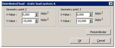
Figure 9 - Definition of a uniformly distributed load.
After drawing all the geometric elements of the model will be as shown in Figure 10.
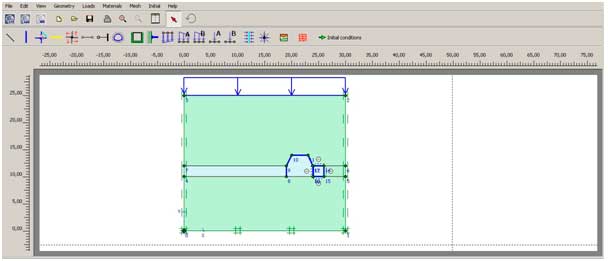
Figure 10 - Geometric model in the data entry box
Material data sets. To simulate the behavior of the soil for a given geometric model to be taken appropriate soil model and its parameters. In Plaxis characteristics of the soil collected in material data sets that are stored in the appropriate database.
Then see the following:
Animation - The total displacement in the model with different penetration security facilities.
(animation developed using Adobe Flash (trial version), 4 frames, 5 cycles of repetition, 644 KB)
Conclusion.
postprocessor software package PLAXIS 2D allows us to derive a significantly greater amount of the calculated results of the model (stress, displacement, strain) but to select a value deepening security structures is enough information presented above. As mentioned above, one of the most important indicators of the underground mine workings is a cross-sectional area at the time of its production operation.
To determine the penetration at which is the best state mines were made to the copy profile section of development, before and after the simulation for different values of emplacement (Pic. 11).
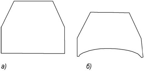
Figure 11 - Steam production: a) before mining model, b) after working model
After determining
sectional area before and after excavation mining models revealed that:
- development without deepening retained 71.4% of the original section;
- development with a deep width of 0.5 security structures retained 81.5% of the original section;
- development with a deep equal to the width of one security structures retained 86.3% of the original section;
- development with a deep equal to 1.5 times the width of guarding structures retained 86.2% of the original section;
- development with a deep equal to twice the width of the security structures retained 76.9% of the original section;
These data plotted changes in the cross section of mountain depending on the uglubki security structures, which shows that deepen ohranooe structure over a depth equal to the width of one security facilities makes no sense (Pic. 12).
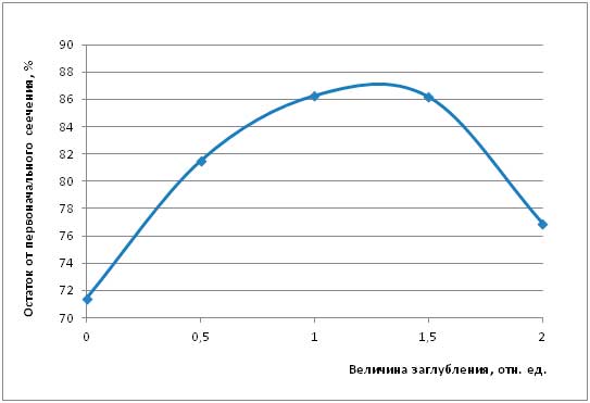
Figure 12 - Changes in the cross section of excavation depending on the security facilities uglubki
But then become meaningless conclusions made earlier about the impact of the stamp deep foundations. Indeed, with the increase of laying up to 2 widths situation worsens.
But in this case there is no error, but only affects that building security is a stamp for the soil, and on the state of production and affects the behavior of the roof rocks. Therefore, reducing the section of development from inception increase security structures explains the negative impact on the state of deep foundations roof generation.
Thus, the results of mathematical modeling established the optimum value of laying rigid security structures, which is the width of 1.0-1.5.
References:
1. В.А.Юдковский, Ю.И.Рудницкий, В.П.Глебов, Бесцеликовая технология охраны и поддержания выработок на шахте «Новодзержинская»// Ежемесячный научно-техн. журнал «Уголь Украины». - 1984. - №10. – с.12.
2. Чакветадзе Ф.А. Разработка эффективных технологий активного воздействия на окружающий массив для повышения устойчивости подземных горных выработок: Автореф. дисс…докт. техн наук: 05.15.02. / МГГУ.– М.– 1994.– 36 с.
3. Спосіб охорони гірничих виробок. Касьян М.М., Негрій С.Г., Мокрієнко В.М., Хазіпов І.В.Пат. № 94327, МПК(2011.01) E21D 11/00 (2006.01), E21С 41/18 (2006.01), опубл. 26.04.2011; 26.04.2010, бюл. № 8– 6с.
4. Медяник В.Ю. Формування склепіння рівноваги над підготовчою виробкою за допомогою смуг змінної жорсткості – як спосіб її охорони і підтримки // Геотехнічна механіка: Міжвід. зб. наук. праць / Ін-т геотехнічної механіки, ім. М.С. Полякова НАН України: VII конференція молодих учених «Геотехнологічні проблеми розробки родовищ, 19 листопада 2009» – Д., 2009. – Вип. 81. – С. 173-183.
5. Уланов А. И. Математическое моделирование геомеханических процессов. Научно-технический вестник Санкт-Петербургского государственного университета информационных технологий, механики и оптики. научная статья, стр. 330-337 С.-Петербург; –2009.
6. Карасев М.А. Эффективное применение численных методов анализа для решения задач геомеханики. Записки Горного института. С. 161-165.2010. Т. 185.
7. Plaxis. Версия 8. Справочное руководство. http://www.plaxis.ru
8. Метод конечных элементов. Материал из Википедии — свободной энциклопедии. http://ru.wikipedia.org/wiki /МКЭ
9. Боровков А.И. и др. Компьютерный инжиниринг. Аналитический обзор - учебное пособие. — СПб.: Изд-во Политехн. ун-та, 2012. — 93 с. — ISBN 978-5-7422-3766-2
10. Система автоматизированного проектирования. Материал из Википедии — свободной энциклопедии. http://ru.wikipedia.org/wiki/cad/cae
11. Моделирование проявлений горного давления / Кузнецов Г.Н., Будько М.Н., Васильев Ю.И., Шклярский М.Ф., Юревич Г.Г.– Л.: Недра, 1968.– 280с.
12. Сучасні проблеми проведення та підтримання гірничих виробок глибоких шахт / Під заг.ред. С.В.Янко.– Донецьк: ДУНВГО, 2003.– 256с.
Introduction.
Before conduct comprehensive laboratory studies necessary to carry out mathematical modeling to establish the possibility of using the proposed technology and the mechanism of squeezing out bedrock security structures of various designs.
In practice calculations using both analytical [ 1 ], and numerical methods [ 2 ]. The first is based on the mathematical methods for solving boundary value problems, usually complex and labor ¬ doemkih and quite often limited by simple geometric shapes of bodies and loading schemes. Numerical methods, which include, in particular, finite difference method, the method of boundary integral equations, boundary element method, finite element method and other methods, in contrast, are not limited to any form of bodies, nor FPIC ¬ bong load application. This, along with the omnipresence of powerful computational techniques you contributes to the diffusion of the engineering environment.
Computational methods:
- finite difference method
- discrete element method
- boundary element method
- Finite Element Method
Finite Element Method (FEM) is currently the standard for solving problems of solid mechanics by means of numerical algorithms.
Actuality.
Once popular method of finite differences, and the claim to universality boundary element method (boundary integral equations) now occupy fairly narrow niche, limited research or special tasks. FEM took the leading position with the ability to simulate a wide range of objects and phenomena. The vast majority of the structural elements, components and structures made of various materials having different natures, can be calculated by the FEM. At the same time, of course, you need to consider inevitable in any numerical approximation of the conventions and error. Therefore, the question of correspondence between the calculated model and reality is perhaps the main using analysis software. Despite the fact that such programs are more or less detailed documentation, they are still to some extent a black box. This means a certain unpredictability of the results, as well as some arbitrariness in their interpretation. Consequently, the quality of the findings made on the basis of results depends entirely on the skill, as well as in relation to the calculation of strength, a fundamental familiarity with the basics of FEM.
Numerical same methods are used to solve complex problems, each of which is almost unique in its boundary conditions, fluid properties. The results of such solutions for a wide range of users are of interest mainly as illustrative ¬ tion efficiency method of solution and to a lesser extent by themselves. Discrete element methods require processor-intensive computer; this limits the length of the model or the number of particles. The finite element method provides an opportunity to take into account in the calculation of different ¬ shaped and complex properties of soils, rather than two indices (E and v or C and φ). FEM thereby stimulated the development of test methods of soils and rocks, and new theories of strength and deformability.
Also, the benefits of FEM include the possibility of reducing the problem to a system of linear or nonlinear algebraic equations directly, without pre-formulation of their differential counterparts. Furthermore the finite element method has attracted the attention of researchers mainly the property that the continuum is broken down into a number of elements that can be considered as a specific part of it. Basic procedures FEM standard and do not depend on the dimension and the type of finite element, which allows for the unification of these procedures and to create software for the calculation of structures and a broad class of applications.
1. Selecting a method of mathematical modeling
Finite element method combined with powerful computer models allow the use of materials of almost any complexity. Thanks FEM have a real opportunity to move to the calculation not only concrete, but concrete structures under complex stress state. Reinforced concrete, as is known, is a complex material consisting of concrete and steel reinforcement working together, but with different mechanical properties. FEM applied to the calculation of reinforced concrete structures is not only a numerical analysis method, but also serves as a simulation tool, when the material model reflects the specificity of the finite element method.
The method FEM discretization object is to solve the equations of continuum mechanics under the assumption that these relations are carried out within each of the elementary regions. These areas are called finite elements. They may correspond to the real part of the space, such as spacing elements, or be a mathematical abstraction elements as bars, beams, plates or shells.
Within Finite element assigned properties, limited to an object area (this can be, for example, the characteristics of rigidity and strength of the material, density, etc.) and describes the values of the field of interest (as applied to the mechanics of this displacement, deformation, pressure, etc.). Parameters in the second group are assigned to the nodes of the element, and then introduced interpolate functions by which the respective values can be calculated at any point within the element or on its boundary. Mathematical description of the problem boils down to the element to tie in knots acting factors. In continuum mechanics, as a rule, travel and effort.
Figure 1 - Three-dimensional finite elements
Figure 2 - Parabolic finite element surface
Figure 3 - Finite elements beams and bar
Algorithm application MKE following:
1. Performed sampling volume occupied part or assembly to the elements, or, as they say, the finite element mesh is constructed. To surround the body region is partitioned into tetrahedra with faces approximated by linear (linear dependence on the coordinates) or parabolic functions of the coordinates. For surface models - on flat (linear) or curved (parabolic dependence) triangles;
2. Finite elements for spatial degrees of freedom are moving in the direction of the axes of the local coordinate system of the element. For end shells to three elements in each node movements are added by three angles of rotation normal to the middle surface region of the approximated element relative to the same axes;
3. Determined according to convert displacements and rotation angles of the nodes to the global coordinate system;
4. Calculated stiffness matrix of finite elements. In the formula for calculating the components of the finite element stiffness matrices addition to the coordinates of nodes includes the elastic moduli and Poisson's ratios of materials. That is, if the assembly is analyzed, then, depending on the details of membership of an element in calculating the stiffness matrices of elements using the appropriate characteristics of the material stiffness;
5. The resulting stiffness matrix using the transition from dependency to local coordinate systems are transformed into global element in the global coordinate system;
6. Stiffness matrix presented in the global coordinates, the union ¬ nyayutsya the global stiffness matrix [ K ];
7. The user-boundary conditions, static and kinematic given to the loads and displacements at the nodes, expressed in the global coordinate system, and are included in the column of effort [ F ];
8. The resulting linear system of equations of the form [ K ] * [ A ] = [ F ] is solved for column movements. This is the most time-consuming step of the calculation. Solutions are used for iterative or direct methods. The stiffness matrix, is typically stored in a compact form, the structure of which is determined before the filling stage of its stiffness matrices of elements;
9. For each finite element, with displacement (rotation angles) at the nodes and the approximating functions are calculated deformation. If linear elements - deformation within the constant elements, if the elements of parabolic - strain vary linearly. On the basis of the voltage computed in the deformation elements. If necessary (software feature) voltage at the nodes of adjacent elements are averaged (this is also a very important stage, are solved differently in different programs), followed by recalculation of stress within each element;
10. Based on the components of the stress-strain state and strength parameters of the material (s), the computation of equivalent stress on any strength criterion.
Quite often modules nonlinear analysis of FEM programs are a superstructure on the base part, responsible for the elastic structural analysis.
Nonlinear problems are characterized by a nonlinear relationship between the operating factors and the response of the system to them. In addition, often the boundary conditions (applied load and displacement) change over time. To account for this phenomenon introduces the concept of time curve. Its meaning is that the input parameter having the dimension of time, and depending on its value, it defines the conditions are assigned. That is actually constructed diagrams in which the abscissa - this time, and the ordinate is power, power, movement, etc. If calculated to contain material, the characteristics of which may be time dependent, the parameter corresponds to the physical time. Otherwise, it is an abstract value, the scope of which is chosen for reasons of convenience representation of curves. In most applications, there are three methods used for different classes of problems.
2 Statement of the problem of modeling
There are many ways of protecting the mines, one of the most effective ways - the construction of the cast strip hardening compositions after stope
Essence of the method: after passing complex purification and extraction of minerals (Figure 4a), erected formwork (Figure 4b), which is placed inside the quick-mix concrete (Figure 4c).
Based on practices used in the construction of buildings - in the presence of soft soil at the base of the foundation to enhance its stability performance inception of the foundation. Decision was made using the software package PLAXIS 2D - working with the finite element method, to test the impact uglubki security structures relative soil, the state generation, as well as to determine the optimal amount of penetration. In PLAXIS 2D software package was created five models of rock mass. One model with standard layout cast strip + four models with varying degrees of penetration of security structures.
Figure 4 - Diagram deepening security structures
3 Creating a mathematical model
After starting the program, a dialog box Create / Open project (Figure 5), where you can open an existing or create a new project.
After selecting "New Project" window appears General settings (General Options), consisting of two tabs Project (Project) and Dimensions (Dimensions) (Figs. 6 and 7).
Figure 5 - Dialog Box Create / Open project
Figure 6 - Project tab window General settings
General Options. The first stage of each task is to set the basic parameters of the finite element model. This is done in the General settings (General Options). These settings include the description of the task, the type of calculation, the basic element type, the basic units and the size of the drawing field. To enter the relevant parameters for the calculation of the foundation, do the following:
In the Title (Name) tab Project (Project), we write the name of the «Model 1»
Figure 7 - Dimensions tab window General settings
In the GeneralType of task (Model) and the type of basic elements (Elements). In the combo box, select Model Plane Strain, and in the Elements - 15-noded (15 angled triangular element).
Under Acceleration (acceleration) indicates the value specified angle gravity equal to -90 º and extending in the vertical direction (down). Apart from the normal gravity values for psevdodinamicheskih calculations can be administered independent of each other acceleration components. Clicking
In the Units (Units) tab Dimensions (Dimensions) leave the default units:
- Length (L) - m (m);
- Force (load) - kN (kN);
- Time (time) - night (day)).
In the Geometry dimensions (geometry) introduced the planned size of the drawing field.
In the Grid (Grid) is defined grid. With the help of a grid on the screen displays a matrix of dots, which can be taken as a starting point. It can also be used for instant reference to the regular points during the creation of a geometric model. The distance between points is determined by the value given in the Spacing (Pitch). The distance between the anchor points may be further divided into smaller intervals by setting field Number of intervals the number of intervals
To confirm settings will click
After completing the general parameters, appears a drafting field with the origin and the direction of the coordinate axes. The X-axis directed to the right, and the axis Y - up. Geometric model can be created anywhere, but within the size of the drawing field. Geometry line - to create objects - (geometric line) is already active. This option can also be selected from the first row of buttons on the toolbar that contains the geometric objects, or from the menu Geometry. With the tool Geometry line traceable region further modeling - By using Plaxis is defined cluster.
Boundary conditions. Boundary conditions can be selected from the second row of the toolbar buttons or menu Loads (loads). To resolve the problems, there are two types of deformation boundary conditions:
- set offset
- load
To set the standard boundary conditions choose Standard fixities (Standard fixing) or menu Loads (Loads) option Standard fixities. As a result of Plaxis create a full consolidation basis of the model (termination), and the vertical boundaries (ux = 0; uy = free) - sliding terminations. Installation in a certain direction will appear on the screen in the form of two parallel lines running perpendicular to this direction (Fig. 9). Thus, moving the movable support are presented in the form of two vertical parallel lines and the solid seal - hatching.
On the upper bound of the simulated array are applying a uniform load of A (Fig. 9). In the task evenly distributed load - sets the amount and direction (Pic. 9).
Figure 9 - Definition of a uniformly distributed load.
After drawing all the geometric elements of the model will be as shown in Figure 10.
Figure 10 - Geometric model in the data entry box
Material data sets. To simulate the behavior of the soil for a given geometric model to be taken appropriate soil model and its parameters. In Plaxis characteristics of the soil collected in material data sets that are stored in the appropriate database.
Then see the following:
Animation - The total displacement in the model with different penetration security facilities.
(animation developed using Adobe Flash (trial version), 4 frames, 5 cycles of repetition, 644 KB)
Conclusion.
postprocessor software package PLAXIS 2D allows us to derive a significantly greater amount of the calculated results of the model (stress, displacement, strain) but to select a value deepening security structures is enough information presented above. As mentioned above, one of the most important indicators of the underground mine workings is a cross-sectional area at the time of its production operation.
To determine the penetration at which is the best state mines were made to the copy profile section of development, before and after the simulation for different values of emplacement (Pic. 11).
Figure 11 - Steam production: a) before mining model, b) after working model
After determining
sectional area before and after excavation mining models revealed that:
- development without deepening retained 71.4% of the original section;
- development with a deep width of 0.5 security structures retained 81.5% of the original section;
- development with a deep equal to the width of one security structures retained 86.3% of the original section;
- development with a deep equal to 1.5 times the width of guarding structures retained 86.2% of the original section;
- development with a deep equal to twice the width of the security structures retained 76.9% of the original section;
These data plotted changes in the cross section of mountain depending on the uglubki security structures, which shows that deepen ohranooe structure over a depth equal to the width of one security facilities makes no sense (Pic. 12).
Figure 12 - Changes in the cross section of excavation depending on the security facilities uglubki
But then become meaningless conclusions made earlier about the impact of the stamp deep foundations. Indeed, with the increase of laying up to 2 widths situation worsens.
But in this case there is no error, but only affects that building security is a stamp for the soil, and on the state of production and affects the behavior of the roof rocks. Therefore, reducing the section of development from inception increase security structures explains the negative impact on the state of deep foundations roof generation.
Thus, the results of mathematical modeling established the optimum value of laying rigid security structures, which is the width of 1.0-1.5.
References:
1. В.А.Юдковский, Ю.И.Рудницкий, В.П.Глебов, Бесцеликовая технология охраны и поддержания выработок на шахте «Новодзержинская»// Ежемесячный научно-техн. журнал «Уголь Украины». - 1984. - №10. – с.12.
2. Чакветадзе Ф.А. Разработка эффективных технологий активного воздействия на окружающий массив для повышения устойчивости подземных горных выработок: Автореф. дисс…докт. техн наук: 05.15.02. / МГГУ.– М.– 1994.– 36 с.
3. Спосіб охорони гірничих виробок. Касьян М.М., Негрій С.Г., Мокрієнко В.М., Хазіпов І.В.Пат. № 94327, МПК(2011.01) E21D 11/00 (2006.01), E21С 41/18 (2006.01), опубл. 26.04.2011; 26.04.2010, бюл. № 8– 6с.
4. Медяник В.Ю. Формування склепіння рівноваги над підготовчою виробкою за допомогою смуг змінної жорсткості – як спосіб її охорони і підтримки // Геотехнічна механіка: Міжвід. зб. наук. праць / Ін-т геотехнічної механіки, ім. М.С. Полякова НАН України: VII конференція молодих учених «Геотехнологічні проблеми розробки родовищ, 19 листопада 2009» – Д., 2009. – Вип. 81. – С. 173-183.
5. Уланов А. И. Математическое моделирование геомеханических процессов. Научно-технический вестник Санкт-Петербургского государственного университета информационных технологий, механики и оптики. научная статья, стр. 330-337 С.-Петербург; –2009.
6. Карасев М.А. Эффективное применение численных методов анализа для решения задач геомеханики. Записки Горного института. С. 161-165.2010. Т. 185.
7. Plaxis. Версия 8. Справочное руководство. http://www.plaxis.ru
8. Метод конечных элементов. Материал из Википедии — свободной энциклопедии. http://ru.wikipedia.org/wiki /МКЭ
9. Боровков А.И. и др. Компьютерный инжиниринг. Аналитический обзор - учебное пособие. — СПб.: Изд-во Политехн. ун-та, 2012. — 93 с. — ISBN 978-5-7422-3766-2
10. Система автоматизированного проектирования. Материал из Википедии — свободной энциклопедии. http://ru.wikipedia.org/wiki/cad/cae
11. Моделирование проявлений горного давления / Кузнецов Г.Н., Будько М.Н., Васильев Ю.И., Шклярский М.Ф., Юревич Г.Г.– Л.: Недра, 1968.– 280с.
12. Сучасні проблеми проведення та підтримання гірничих виробок глибоких шахт / Під заг.ред. С.В.Янко.– Донецьк: ДУНВГО, 2003.– 256с.