Abstract
Contents
Introduction
Relevance of the master's work topic
The scientific innovation of the work
Expected practical results
Object and subject of research
Point, Line and Edge Detection
Gradient Operators
The Laplacian
Edge Linking and Boundary Detection. Local Processing
Basic Global Thresholding
Region growing
Segmentation by Morphological Watersheds
The Use of Motion in Segmentation. Spatial Techniques
Conclusions
References
Research of image segmentation methods
Introduction
Segmentation subdivides an image into its constituent regions or objects.
The level to which the subdivision is carried depends on the problem being
solved. That is, segmentation should stop when the objects of interest have
been isolated.
Segmentation of nontrivial images is one of the most difficult tasks in image
processing. Segmentation accuracy determines the eventual success or failure
of computerized analysis procedures.
Relevance of the master's work topic
Segmentation of video frames is very important in the video data digital
processing. This procedure is applied at the stage of frame generation.
There are three types of frames used in video compression: I‑frames
(Intra), P‑frames (predicted), and B‑frames (bidirectional). An I‑frame
is an 'Intra-coded picture', in effect a fully-specified picture, like a
conventional static image file. P‑frames and B‑frames hold only the
changes in the image. And these changes aren’t applied the whole frame,
but to each slice of picture. So there is a need to segment intraframe
into slices to achieve good compression rate.
The scientific innovation of the work
The scientific innovation of this work is to develop an improved
segmentation method of video sequence frame.
Expected practical results
As a result of research it's expected to achieve optimal layer
separation of keyframe for generating following reference frames.
Object and subject of research
The object of research is the image frame sequences containing different
fragments. The subject of research is the method of image
segmentation into layers or regions.
Main results
Point, Line and Edge Detection
Image segmentation algorithms generally are based in on one of two basic
properties of intensity values: discontinuity and similarity. Let’s
begin with the methods suitable for detecting gray-level discontinuities
such as points, lines, and edges. The most common way to look for
discontinuities is to run a mask through the image.
 (1.1)
(1.1)
The detection of isolated points in an image is straightforward in
principle. For example, 3x3 mask is used:
| -1 |
-1 |
-1 |
| -1 |
8 |
-1 |
| -1 |
-1 |
-1 |
Figure 1.1. A general 3х3 mask.
Point has been detected at the location on which the mask is centered if
 (1.2)
(1.2)
where T is a nonnegative threshold and R is given by Eq. (1.1). This
formulation measures the weighted differences between the center point
and its neighbors. The idea is that an isolated point will be quite
different from its surroundings. Mask coefficients sum to zero,
indicating that the mask response will be zero in areas of constant gray
level.
For line detection such masks are used:
|
|
|
|
|
| Horizontal |
+45 |
Vertical |
-45 |
Figure 1.2. Masks for line detection.
The response will be the most strong to lines one pixel thick. Each mask
sets the line direction. Coefficients in each mask sum to zero. It is
possible to vary lines thick.
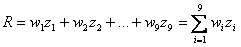
Edge detection is the most common approach for detecting meaningful
discontinuities in gray level. Models of ideal and ramp digital edges:
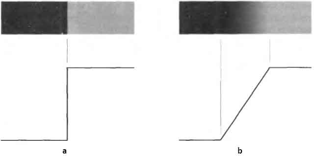
Figure 1.3. (a) Model of an ideal digital edge;
(b) model of an ideal digital edge.
The degree of an image edge blurring is determined by factors such as
the quality of the image acquisition system, the sampling rate, and
illumination conditions under which the image is acquired. Figure 1.4
shows horizontal gray-level profile of the edge, its first and second
derivatives. The first derivative is positive at the points of
transition into and out of the ramp as we move from left to right along
the profile; and is zero in areas of constant gray level. The second
derivative is positive at the transition associated with the dark side
of the edge, negative at the transition associated with the light side
of the edge, and zero along the ramp and in areas of constant gray
level.
It’s possible to conclude that the magnitude of the first derivative can
be used to detect the presence of an edge at a point in an image.
Similarly, the sign of the second derivative can be used to determine
whether an edge pixel lies on the dark or light side of an edge.
Note two additional properties of the second derivative around an edge:
(1) It produces two values for every edge in an image (an undesirable
feature); and (2) an imaginary straight line joining the extreme
positive and negative values of the second derivative would cross zero
near the midpoint of the edge. The zero-crossing property of the second
derivative is quite useful for locating the centers of thick edges.
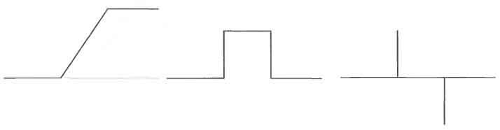
Figure 1.4. Horizontal gray-level profile of the
edge, its first and second derivatives.
Real images are often corrupted by noise.
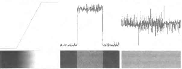
Figure 1.5. Gray level profile of a ramp edge
corrupted by noise; noise effects on first and second derivatives.
Gradient Operators
The gradient of an image f(x, y) at location (x, y) is defined as the
vector
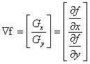 (1.3)
(1.3)
Magnitude of this vector
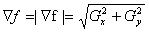 (1.4)
(1.4)
This quantity gives the maximum rate if increase of f(x, y) per unit
distance.
The direction of the gradient vector
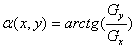 (1.5)
(1.5)
Computation of the gradient of an image is based on obtaining the
partial derivatives df/dx and df/dy at every pixel location. First-order
partial derivatives can be computed by:
а) Roberts cross-gradient operators: : Gx = (z9-z5);
Gy = (z8 – z6);
б) Prewitt operators: Gx = (z7+z8+z9) – (z1 + z2 + z3);
Gy = (z3+z6+z9) – (z1 + z4 + z7);
в) Sobel operators : Gx = (z7+2*z8+z9) – (z1 + 2*z2 + z3);
Gy = (z3+2*z6+z9) – (z1 + 2*z4 + z7).
| z1 |
z2 |
z3 |
| z4 |
z5 |
z6 |
| z7 |
z8 |
z9 |
|
|
|
| Image region |
Roberts |
Figure 1.6. Image region and different masks for
computation of the gradient.
Masks of size 2x2 are awkward to implement because they do not have a
clear center. The Prewitt masks are simpler to implement than the Sobel
masks, but the latter have slightly superior noise-suppression
characteristics, an important issue when dealing with derivatives.
An approach used frequently is to approximate the gradient by absolute
values:
 (1.6)
(1.6)
The Laplacian
The Laplacian of a 2-D function f(x, y) is a second order derivative
defined as
 (1.7)
(1.7)
For a 3x3 region, one of the two forms encountered most frequently in
practice is
 (1.8)
(1.8)
A digital approximation including the diagonal neighbors given by
 (1.9)
(1.9)
|
|
| -1 |
-1 |
-1 |
| -1 |
8 |
-1 |
| -1 |
-1 |
-1 |
|
Figure 1.7. Laplacian masks for equations (1.8)
and (1.9)
Edge Linking and Boundary Detection. Local Processing
One of the simplest approaches for linking edge points is analyze the
characteristics of pixels in a small neighborhood (3x3 or 5x5) about
every point (x, y) in an image that has been labeled an edge point by
one of the techniques discussed in the previous section. All points that
are similar according to a set of predefined criteria are linked,
forming an edge of pixels that share those criteria.
 (1.10)
where E is a nonnegative threshold.
 (1.11)
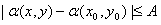
where A is a nonnegative angle threshold. The direction of the edge at
(x, y) is perpendicular to the direction of the gradient vector at that
point.
A point in the predefined neighborhood of (x, y) is linked to the pixel
at (x, y) if both magnitude and direction criteria are satisfied. This
process is repeated at every location in the image.
Basic Global Thresholding
The simplest of all thresholding techniques is to partition the image
histogram by using a simple global threshold T.
The following algorithm can be used to obtain T automatically:
1. Select an initial estimate for T.
2. Segment the image using T. This will produce two groups of pixels:
G1 consisting of all pixels with gray
level values > T and G2 consisting of pixels with values >=T.
3. Compute the average gray level values µ1 and µ2 for the pixels in regions G1 and
G2.
4. Compute a new threshold value: T = (µ1 + µ2) / 2.
5. Repeat step 2 through 4 until the difference in T in successive iterations is
smaller than a predefined parameter T0.
Region growing
Region growing is a procedure that group pixels or subregions into
larger regions based on predefined criteria. The basic approach is to
start with a set of “seed” points and from these grow regions by
appending to each seed those neighboring pixels that have properties
similar to the seed.
Selecting a set of one or more starting points often can be based on the
nature of the problem. The selection of similarity criteria also depends
on the type of image data available.
The problem in region growing is the formulation of a stopping rule.
Basically, growing a region should stop when no more pixels satisfy the
criteria for inclusion in that region. Additional criteria that increase
the power of a region-growing algorithm utilize the concept of size,
likeness between a candidate pixel and the pixels grown so far, and the
shape of the region being grown.
Segmentation by Morphological Watersheds
The concept of watersheds is based on visualizing an image in three
dimensions: two spatial coordinates versus gray levels. In such a
“topographic” interpretation, three types of points: (a) points
belonging to a regional minimum; (b) points at which a drop of water, if
placed at the location of any of those points, would fall with certainly
to a single minimum; and (c) points at which water would be equally
likely to fall to more than one such minimum. For a particular regional
minimum, the set of points satisfying condition (b) is called the
catchment basin or watershed of that minimum. The points satisfying
condition (c) form crest lines on the topographic surface and are termed
divide lines or watershed lines.
The basic idea is simple:
suppose that a hole is punched in each regional minimum and that the
entire topography is flooded from below by letting water rise through
the holes at a uniform rate. When the rising water in distinct catchment
basins is about to merge, a dam is built to prevent the merging. These
dam boundaries correspond to the divide lines of the watersheds.
Figure 1.8. Image segmentation by morphological
watersheds.
The Use of Motion in Segmentation. Spatial Techniques
One of the simplest approaches for detecting changes between two frames
f (x, y, ti) and f (x, y, tj), is to compare two images pixel by pixel.
One procedure for doing this is to form a difference image. Such image
includes only nonstationary components.
A difference image may be defined as
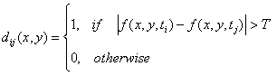 (1.18)
where T is a specified threshold. dij(x, y) has a value of 1 at spatial
coordinates (x, y) only if the gray-level difference between the two
images is appreciably different at those coordinates, as determined by
T.
In dynamic image processing, all pixels in dij(x, y) with value 1 are
considered the result of object motion. This approach is applicable only
if the two images are registered spatially and if the illumination is
constant. In practice, 1-valued entries in dij(x, y) often arise as a
result of noise. Such isolated points may be ignored.
Consider a sequence of image frames f(x, y, t1), f(x, y, t2),…, f(x, y,
tn) and let f(x, y, t1) be the reference image. An accumulative
difference image (ADI) is formed by comparing this reference image with
every subsequent image in the sequence. A counter for each pixel
location in the accumulative image is incremented every time a
difference occurs.
Often useful is consideration of three types of accumulative difference
images: absolute, positive, and negative ADIs. Let R(x, y) denote the
reference image and let k denote tk, so that f(x, y, k) = f(x, y, tk).
We assume that R(x, y) = f(x, y, 1). Then, for any k > 1, and keeping in
mind that the values of the ADIs are counts, we define the following for
all relevant values of (x, y):
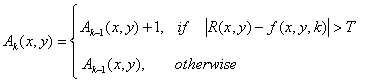 (1.19)
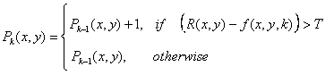 (1.20)
 (1.21)
These ADIs start out with all zero values (counts). ADIs are the same
size as the images in the sequence.
Figure 1.9. Absolute, positive, and negative ADIs.
In practice, obtaining a reference image with only stationary elements
is not always possible, and building a reference from a set of images
containing one or more moving objects becomes necessary.
Conclusions
The above material shows that there are many methods for image
segmentation. While the list of described methods isn’t exhaustive,
these methods are typical representatives of the segmentation technique.
You can also come to the conclusion that different techniques can be
combined. For example, it is possible to combine the spatial
segmentation with the segmentation of moving objects.
References
-
R.C. Gonzalez, R.E.Woods, Digital Image Processing, Prentice-Hall, Inc,
Upper Saddle River, New Jersey, pp. 567-642, 2002.
-
Segmentation (image processing) [Электронный ресурс] –
Режим доступа к статье:
http://en.wikipedia.org/wiki/Segmentation_(image_processing)
-
Универсальная классификация алгоритмов сегментации изображений [Электронный ресурс]
/ С.В. Поршнев, А.О. Левашкина – Режим доступа к статье:
http://www.jurnal.org/articles/2008/inf23.html
-
D.J.Williams and M.Shas. “Edge Contours Using Multiple Scales”.
Computer Vision, Graphics and Image Processing, 51, 1990,
pp.256-274.
-
V. Lacroix. “The Primary Raster: A Multiresolution Image
Description”. In Proceedings of the 10th International Conference on
Pattern Recognition, 1990, pp. 903-907.
-
J.F.Canny. “A Computational Approach to Edge Detection”. IEEE
Transactions on Pattern Analysis and Machine Intelligence, 8(6), Nov
1986, pp. 679-698.
-
D. Ziou and S. Tabbone. “A Multi-Scale Edge Detector”. Pattern
Recognition, 26(9), 1993, pp.1305-1314.
-
T. Lindeberg. “Edge Detection and Ridge Detection with Automatic
Scale Selection”. In Proceedings of IEEE, International Conference
on Computer Vision and Pattern Recognition, San Francisco, 1996, pp.
465-470.
-
William K. Pratt Digital Image Processing,
Wiley-Interscience Publication, 2001, pp. 551-589.
-
L. M. J. Florack, B. M. ter Haar Romeny, J. J. Koenderink, and M. A.
Viergever. “Scale and the diferential structure of images”. Image
and Vision Computing, 10(6), Jul 1992, pp.376-388.
|