Summary on the final work

1 Introduction

2 Analysis of task partitioning space using a treemap

    2.1 Treemap as a method of displaying information

    2.2 Parameters for evaluating the effectiveness of the partition of the space treemap

3 Review of existing algorithms for partitioning space using a treemap

    3.1 Slice-and-dice algorithm

    3.2 Squarified treemap

    3.3 Ordered treemap

    3.4 Strip treemap

    3.5 Quantum treemap

4 Conclusions. Goals and objectives for further research

5 Literature

1 Introduction

Studing relationships and patterns in geospatial data is a difficult task because of their huge size. Data can be of different nature and from different sources. There is a need to develop methods for effective interaction and computer-processing and human vision, methods for data analysis and visualization, enabling detection of dependencies, the formulation of hypotheses and extracting knowledge from the data.

Geovizualization – a method of investigation of spatial knowledge, hidden in multidimensional geographical and temporal data through interaction with a map or graph. Geovizualization is not just a passive process of viewing and reading maps. This is an active process that involves sorting, selection, filtering and converting data to determine the dependencies and relationships. Maps and graphs in this context do more than "show data", they are active instruments in the process of user thinking [1].

Approaches to geovizualization

Traditional approaches used in geovizualization is a direct mapping of each entry from an array of data, then an analyst examines the data and tries to fing the correlation in the data. However, the amount of sources and data grows every day, what makes it more difficult for the analyst. Presentation of data (paper, screen or other device) may become illegible due to visual overload, large amounts of data and information of different nature. The user may have problems perceiving, tracking and understanding a set of visual elements, which vary simultaneously. Many methods have been developed for the visual analysis of spatial data through direct mapping. However, it is unlikely that these methods can effectively solve the problem of congestion in the data. Approaches in geovizualization to display large amounts of data:

- mapping and visualization of an abstract set of data obtained from the preliminary data processing;

- development of various ideas for using space more efficiently maps.

Among the main methods of data preprocessing are:

- the construction of the correlation matrix and determination of relevant factors;

- cleaning and data transformation;

- factor analysis, principal component analysis;

- sorting, aggregation, filtering, etc.

Methods for using space more efficiently maps include:

- density map;

- bar graphs, charts, graphs, time series;

- Animation;

- space-time cube;

- ring maps, tree maps, etc.

In general, the process geovizualization shown in Fig. 1: The base of the pyramid is the raw data domain, because of their huge size they are very difficult to analyze and work with them. Tip of the pyramid is data received after geovizualization: there is much less data and the user's attention is focused on what matters for decision.

Figure 1 – Process of geovizualization

This paper will consider tree-maps, their effectiveness when displaying large amounts of data and their applications.

Relevance of work:

Treemaps are used to display a wide range of data of hierarchical nature. NewsMap – online application that displays Google News in a treemap. Color of the rectangle determines the type of news, and its size – the number of articles on the Internet on this topic. Another very good example of using treemaps is a "market map" on the site Smartmoney.com. In this application, companies are divided into different regions, depending on market sectors in which they reside. The size of each rectangle, which characterizes the company depends on its market share. Color rectangles also carries information, and is in the range from red to green, it is responsible for the dynamics of growth or decline of a company or the scope of the market as a whole. Also there are many applications using treemaps for:

- mapping the file system;

- display of photographs;

- medicine, mapping the human genome;

- Data conversion from Ecxel into a treemap;

2 Analysis of task partitioning space using a tree-map

Treemap – a method of displaying large hierarchical data. They effectively combine the Venn diagrams and pie charts. Originally designed to display the files on your hard drive, now tree-maps are used in many industries ranging from financial analysis and ending with sport reviews and medicine [2].

2.1 Treemap as a method of displaying information

Ben Shniderman invented a new presentation of data as a treemap for a visual representation of the file system of his computer. The traditional approach to display tree structures shows nodes and levels of hierarchy as folders and connecting arrows (Fig. 1). It works and is pretty good, for tree structures of small size. However, if the same approach is applied to trees larger, with hundreds or thousands of nodes and many levels of hierarchy, chaos appears on screen as a set of folders and lines.

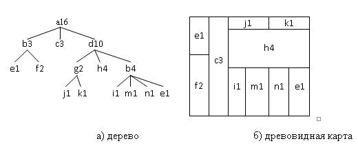
In the beginning, treemap consists of one large rectangle, and then there is a division of the rectangle into regions smaller recursively. The initial rectangle is the root of the tree. It is divided into a set of smaller rectangles separated horizontally, each of whom is a child of the root of the tree. The process is then repeated at each level of hierarchy the direction of separation varies from horizontal to vertical, and vice versa [5].

Figure 2 – The traditional data mapping tree structure

Fig. Figure 2 shows the transformation of the data presented in the form of a tree to a treemap.

Figure 3 – Data conversion: tree to treemap

At this point in the treemap, the following approaches are used to show the information:

- the size of the rectangles;

- color rectangles;

- annotations.

Displaying trees in a treemap has 2 advantages. Firstly, this is something that is very easy to see, a hierarchical structure, shows the links between levels. Child levels are within its parent. Another advantage is that with this representation, the space map is used very effectively. The initial rectangle is completely filled with boxes of smaller size.

Tree map is especially effective way of displaying trees if each leaf of the tree has a weight associated with it. As the weight can be: file size, in Shniderman case, physical weight, monetary value, sugar, etc. Depending on the weight of a leaf, it will take more or less space on the map [3].

2.2 Parameters for evaluating the effectiveness of the partition of the space treemap

Key aspect in the creation of treemaps is the algorithm used to create nested rectangles that make up the card. The effectiveness of the algorithm is determined by the following parameters:

- the average ratio of the rectangles (the average coefficient of proportionality);

- dynamic coefficient of variation;

- the readability of the map;

- ordering information.

Average coefficient of proportionality is determined by the formula:

- AAR (Average Aspect Ratio)

- l – width of the rectangle;

- h – the height of the rectangle;

- n – total number of rectangles.

The closer the coefficient of proportionality of a single box to 1, the closer its shape to a square. And, accordingly, the closer the average coefficient of proportionality to 1, the more "square" is the map. It's difficult fo people to work with the elongated rectangle: Rectangles with different coefficients of proportionality are difficult to compare with each other, add annotations, and even just to see on the map.

Average dynamic coefficient of change is determined by the formula:

- ADCH (Average Dynamic Coefficient of Change)

- n – total number of rectangles;

- R – rectangle, defined by 4 numbers (x, y, w, h);

- d (R1, R2) – the distance between the rectangles is determined by the formula:

- x1, y1 – coordinates of the upper-left corner of the 1st rectangle;

- w1, h1 – coordinates of the lower-right corner of the 1st rectangle;

- x2, y2 – coordinates of the upper left corner of the 2nd rectangle;

- w2, h2 – coordinates of lower right corner of the 2nd of the rectangle;

Dynamic coefficient of change describes how the structure of rectangles of one map is different from another. And, therefore, than this ratio is lower, the better: small changes in the data lead only to small rebuild of the map.

We choose "unweighted" average coefficient of proportionality and of dynamic change, that is, rectangles with a small area of influence on these factors, just as large ones. An alternative might be to use a "weighted" factors, as rectangles Larger contribute more to the overall visual presentation. But the problem with elongated rectangle is more typical of smaller rectangles, and often degrade the proportionality of large rectangles in favor of small ones. The use of "weighted" factors leads to the formation of small, elongated rectangles [10].

Another parameter that determines the efficiency of the algorithm is easier to read maps – a metric that characterizes how easily and quickly, you may find the rectangle you are looking for. This metric is much more difficult to measure mathematically. Readability depends on the consistency and predictability of layout map. Sequence in the data allows a person to follow the pattern quickly, without jumping from place to place. The predictability of the user's eye focuses on the region where, in his view, the rectangle is located. There are several approaches to measure this metric:

- an experiment: show users the same data, grouped in different ways (on different algorithms) and related tasks to find the desired rectangle. Readability, then, can be measured through interviews and analysis of search time;

- Tracking the movement of the human eye while viewing the map. The more often a person changes the direction of viewing the map or jump from place to place, the worse is the readability. This approach is more mechanical and requires no further interview after viewing the map.

Each map is assigned a numeric value for readability and shows how easily a user can find an interesting rectangle.

Tree maps can be ordered and unordered. For most real data, order is important and it carries an important piece of information, so another important property, determining the effectiveness of maps, is the ordering of the data.

3 Review of existing algorithms for partitioning space using a tree-map

Key moment, a place where the most algorithms are different, is the calculation the boundaries of the rectangles. The majority of algorithms are based on a consistent pattern,– which handles only one node at each step. There are algorithms that look ahead a list of child nodes and their placement, in determining the boundaries of the rectangle. However, the main idea of all the algorithms remains the same: a function that processes each node, depending on its size, will allocate the appropriate amount of space. If the node contains child nodes – they are placed inside the parent.

Most widely-used algorithms partition of the space treemaps are those ones:

- Slice-and-dice;

- squarified algorithm;

- cluster algorithm;

- pivot-by-middle;

- pivot-by-size;

- pivot-by-split-size;

- strip treemap.

3.1 Slice-and-dice algorithm

The first algorithm proposed by B. Shniderman was traditional algorithm slice-and-dice. The space of the map is divided into sub-rectangles, each level of hierarchy the orientation of lines (horizontal or vertical) is changed. An example of the transformation of the tree and display it in a tree map, using the algorithm of slice-and-dice is shown in Fig. 4.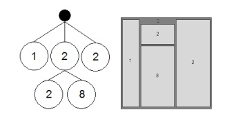

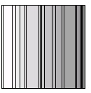
Figure 5 – Transformation of a tree in a tree-map, algorithm slice-and-dice

This algorithm is easy to implement and it is quite effective for small data size, but with the data of big size, the algorithm often leads to the formation of a large number of elongated rectangles. This problem is shown in Figure 5 – a very large number of elongated rectangles, which are difficult to work with [9].

Figure 6 – Slice-and-dice algorithm

Strengths of this algorithm are the characteristics of the "coefficient of dynamic change" and "readability." It also preserves the ordering of elements. However, due to a very high coefficient of proportionality is very rarely used in practice as it is, more often it serves as a measure of comparison to other algorithms.

Estimation of the complexity of the algorithm:

Treemap can be constructed in one pass of the algorithm on a tree. Therefore, assuming that the calculation of the size and color of the rectangle is consonant, run time O(n), where n – the number of nodes in the tree.

3.2 Squarified treemap

How can we break the starting area on the sub-rectangles of smaller size so that the average coefficient of proportionality was as close to 1? A list of all possible allocations is very large and this problem belongs to the class NP-hard problems. However, based on the algorithm of the squarified map is not an exhaustive search, no need to find the optimal solution, it is necessary to obtain a good solution in a short computing time [4].

The algorithm of the squarified treemap is:

- a partition for all the sublevels are not made simultaneously. This leads to a significant increase in computing time. Instead, each level deals only with the coming child nodes, and made their accommodation,so the average aspect ratio for this level is close to 1. At the next level of the hierarchy, there will be the initial rectangle with aspect ratio close to 1, and therefore a good starting point for placement of child nodes. The process is then repeated recursively;

- rectangles along the lines of the free space as long as the worst (highest) proportionality of all the rectangles in this line continues to shrink. Once the worst-case proportionality factor reaches its minimum, and adding a rectangle leads to an increase in the worst-case coefficient of proportionality, placement of this line is completed, proceed to the next.

Example:

Suppose we have a rectangle with width 6 and height 4, and the rectangle should be divided into smaller rectangles of area 6, 6, 4, 3, 2, 2 and 1. The result of traditional slice-and-dice algorithms is shown in Fig. 6, formed by a set of elongated rectangles with aspect ratio 16 and 36, respectively.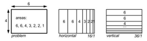

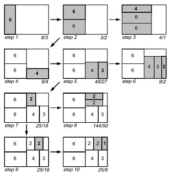
Figure 7 – Result of slice-and-dice algorithm

First step of the algorithm is a partition of the initial rectangle. Selects the horizontal partition, because the width is greater than height. Then, one more rectangle is added(Fig. 7). The coefficient of proportionality first rectangle 8 \ 3. Then, we add the second rectangle over the first. The proportionality coefficient is improved to 3 / 2. Add a third rectangle, but the proportionality factor deteriorating to 4 / 1. Therefore, we believe that we have found the optimal solution of the left half in step 2 and proceed to the decomposition of the right half.

As the initial partition has been selected vertical, since the width greater than height. In step 4, if we add a rectangle with an area of 4, and then with an area of 3 to step 5, the proportionality factor is improved. Adding the next rectangle with an area of 2 does not improve the result, so we believe the result at step 5 the best and go to partition the upper right of the rectangle.

Process is repeated until all rectangles are placed. The result of the squarified partition algorithm is shown in Figure 7

Figure 8 – Result of the squarified partition algorithm

The algorithm does not guarantee an optimal solution and you can come up with counterexamples. Also, the sequence of placement of rectangles is important. Usually better to start with the largest rectangles, arrange them is the most difficult.

Disadvantages of the squarified and cluster treemaps:

- The slightest change in data leads to a significant restructuring of the rectangles map. These changes are immediately visible to eye, and it is very difficult for a person to trace the dynamics of change in the data, with constant changes in layout (structure) of the map;

- These algorithms do not preserve the ordering of the data, hence the readability of these algorithms is also very low.

Estimation of the complexity of the algorithm:

First rectangles are sorted by size, which takes time O(n * logn). Runtime remainder of the algorithm depends on the average number of rectangles in each row. Since the dimensions of the rectangle in the current row must be recalculated every time you add a new rectangle to the line time is obtained by O (n * logn) + O (n * B (n)), where B (n) – the average number of rectangles in a row. Thus, the execution time is bounded below by O(n * logn), if O (B (n)) <= O(n * logn). In the worst case, when all the rectangles are in the same line (B(n) = n), run time is O(n * n), which is the upper bound of execution time. On average, however, each line will contain vn rectangles, and the average time O(n * vn).

3.3 Ordered treemap

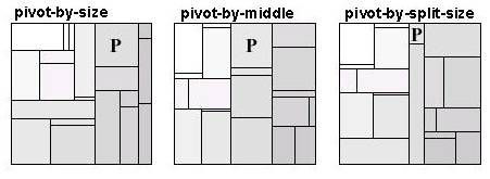
Main feature of this algorithm is that it is possible to create a layout map of the space in which the data following each other will be located close to each other. Despite the fact that the layout is not a simple linear sequence, as for slice-and-dice algorithm, it creates limitations and because of this map is rearranged slightly by changes in the data [6].

The algorithms of this class characterized by a partial ordering of elements.

The basis of ordered maps, starting from the rectangle R, which is to be divided. Input is a list of items ordered by the index and having different sizes. Specific element (reference – pivot) is chosen and placed on the initial rectangle R, the square (the coefficient of proportionality is 1). The remaining elements are placed in 3 large rectangles, which form the unused space rectangle R. The algorithm is recursively applied to each of the 3 rectangles.

There are several algorithms for ordered treemaps:

- pivot by middle;

- pivot by size;

- pivot by split size.

For the algorithm "the pivot on the size" as the reference element is chosen element of the largest size, the largest element is usually the most difficult to place, so it is better to start from it when the entire map is free. The idea of the algorithm is shown in Fig. 8.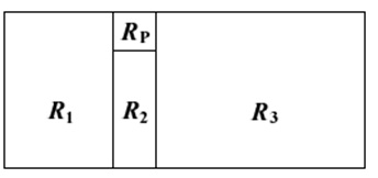

Figure 9 – Ordered treemap

Algorithm:

1. Choose the pivot P, the largest in size.

2. If the width of the initial rectangle R is greater than or equal to the height, divide R into 4 rectangles R1, Rp, R2 and R3, as shown in Fig. (Otherwise, if the width is less than the height, change the axis, y = x);

3. Sort P in the rectangle Rp, the exact size of which will be defined in step 4.

4. Divide all the items in the list except the P to 3 groups L1, L2, L3, to add to the rectangle R1, R2 and R3. L1 and L3 can be empty. Assume that the group consists of L1 elements with index less than P. Put that in the group of L2 for all elements of the index is less than in group L3 and the proportionality factor P as close to 1.

5. Recursively place the L1, L2 and L3 (if they are not empty) rectangles R1, R2, R3, in accordance with the algorithm.

Algorithm "pivot by size" is almost identical to the above, the difference lies in the fact that as a reference element is chosen is not the largest element, but simply a central element (i.e, if the sequence consists of n elements as the reference element will be selected with index n / 2) [7].

For the algorithm "pivot by split size" reference element is chosen so that the total area of rectangles to be placed in regions R1 and R3 is nearly the same.

Results of algorithms "pivot by middle", "pivot by size" and "pivot by split size" is shown in Fig. 9.

Figure 10 – Comparison of ordered treemaps

Ordered tree maps occupy an intermediate position, the average coefficient of proportionality of the rectangles that make up the map is much lower than the traditional slice-and-dice algorithm, but not so low as to cluster and squarified tree maps. They vary much more smoothly than cluster and squarified maps, but not as smoothly as traditional maps, which are based on an slice-and-dice algorithm. Thus, the ordered tree maps are a good choice when the coefficients of proportionality, the dynamic changes and readability, all are important requirements.

Evaluating the effectiveness of the algorithms:

For algorithms "pivot by size" and "pivot by split size» – O(n * logn) the average and O(n * n) at worst.

Algorithm "pivot by middle» – O(n * logn) in the worst case.

3.4 Strip algorithm

Strip algorithm is a modification of an existing tree algorithm of squarified maps. It is based on an ordered processing sequence of rectangles and place them into strips (vertical or horizontal) of different widths (Fig. 10).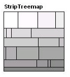

Figure 11 – Strip treemap algorithm

This algorithm dynamically changes the width of the current strip of rectangles. It provides better readability than the traditional algorithms that underlie the ordered treemaps and comparative proportionality factors and the dynamic changes [8].

Algorithm:

Input data is the initial region R for the separation and consistency of child rectangles of a certain size, ordered by index. We continue to add rectangles to the current line up as long as the average coefficient of proportionality of all the bars that line reduced. With its increasing, start a new line. Every time you add a new rectangle to the line, the sizes of all the rectangles of the line dynamically recalculated, and changes its thickness.

The steps are:

- scale the total area of all rectangles, so it was equal to the square of the initial rectangle.

- Create a new line – the current line.

- Add a rectangle to the current line, count the thickness of the line on the basis of all the rectangles line, then recalculate the width of each rectangle line.

- If the average coefficient of proportionality of the current line has increased, while adding the rectangle in step 3, delete the rectangle from the line, move it back to the list of rectangles to process and go to step 2.

- If all the rectangles are processed – the end, otherwise – to step 3.

This algorithm is a simplified version of the squarified partition algorithm. In the quadratic algorithm, rectangles are sorted by size, which improves the coefficient of proportionality, but lost the ordering of elements. Also, for a squarified, as opposed to strip, the algorithm adds rectangles both horizontally and vertically, which again improves the coefficient of proportionality, but degrades readability.

Strip algorithm works well, but often there is a problem with the placement of the last line, since the decision to add the rectangle to the line is based only on the average ratio of the rectangles of the current line. Therefore, you might get a long thin line at the very end, and the remaining rectangles, which, as a result will be very stretched.

This problem can be solved if we add the prediction and treatment of the following lines beforehand. After processing the current line is the next line, and compared the coefficients of proportionality, if the rectangles of the next line will be moved to the current line. If the average proportionality factor of 2 lines below when you move the rectangles of the next line in the current, they are moved.

Evaluating the effectiveness of the algorithm:

For each rectangle is calculated the average coefficient of proportionality of the current line. In each row, on average, squareRoot(n) rectangles. Therefore, the average run time – O(squareRoot(n)).

3.5 The quantum treemaps

All the above algorithms use the following ways to show the information :

- the size of the rectangles;

- color of the rectangles;

- annotations.

Quantum treemaps use another way to convey the information: rectangles contain visual information, such as photographs or images [8]. Example of quantum tree maps shown in Fig. 11.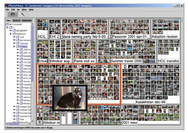

Figure 12 – Quantum treemap

Problem of using the traditional algorithms for displaying visual information is that, as a rule, images have a fixed size, while most algorithms, creates tree map with rectangles, whose size is dynamically adjusted. Therefore, they are not suitable for displaying this kind of information. The solution may be scaling the picture in a rectangle, but with such an approach area of the map is not used effectively – there is a lot of empty areas. Example of tree maps, using algorithms and quantum-ordered tree-maps shown in Fig. 12.

Figure 13 - Ordered and quantum tree maps

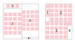
Free space still occurs, but it is much less while using quantum treemaps.

4 Conclusions. Goals and objectives for further research

Promising directions for the development of treemaps are:

- optimization of ordered treemaps, improving the coefficient of proportionality;

- optimization of the cluster and squarified tree maps, improving the dynamic changes;

- study of the layout algorithms to combine their strengths: global stability – local readability;

- formulation of the theorem which characterizes the dependence of the proportionality coefficient and the dynamic changes. They are characterized by an inverse relationship;

- the study of 3-dimensional treemaps;

- finding new ways of passing information: animation, textures, sounds, lines, images and other perceptual techniques.

Main objectives of this work:

- define the scope of tree maps;

- assess the effectiveness of treemaps as a geovizualization method for displaying spatial-temporal and abstract data;

- develop more effective methods of partition of treemap space.

5 Literature

1. Dodge M., McDerby M., Turner M. Geographic visualization. Concepts, tools and applications, 2008.-p. 1-9.
2. Slingsby A., Dykes J., Wood J. Using treemaps for variable selection in spatio-temporal visualization, 2008.-p. 1
3. Shneiderman B. Treemaps for space-constrained visualization of hierarchies, 1998-2009 .- p. 1-10.
4. Bruls M., Huizing K., Jarke J. Squarified treemaps, 2000. - P. 3.
5. Kerwin T., Survey of treemap techniques, 2001.
6. Shneiderman B., Wattenberg M., Ordered Treemap Layouts, 2000.
7. Engdahl B., Ordered and Unordered Treemap Algorithms and Their Applications on handheld devices, 2005.
8. Bederson B., Ordered and Quantum Treemaps: Making Effective Use of 2D Space to Display Hierarchies, 2002.
9. Lu H., Fogarty J., Cascaded Treemaps: Examining the Visibility and Stability of Structure in Treemaps, 1999.
10. Slingsby A., Using treemaps for variable selection in spatio-temporal visualisation, 2008.

Important

When writing this master of the abstract work is not completed yet. Final Completion: December 2011 Full text of the work and materials on the subject can be obtained from the author or his manager after that date.