|
For the ODE systems of the dimension m form of difference equations of type (4.2) is defined by the formula (7.1). This
formula assumes relation of calculated factors to the n-th block.
 (7.1) (7.1)
By the analogy with the formulation of Cauchy problem (4.1), following facts are assumed with respect to the ODE system:
- initial values u0,j definition for the 1-st block;
- initial values u0,j for other blocks (n > 1) are calculated in previous blocks (n–1).
For the ODE system solving iterative process (7.2) is used for a preliminary stage. Iterative process (7.3) is used for
direct iterations performing for the approximate solution calculation [5].
 (7.2) (7.2)
 (7.3) (7.3)
Let the numerical calculation process of required function values is performed on k points of the grid. Let
the processor unit with number i performs approximate solution calculation
 in the fixed point ti for all equations of the original system. In order to realize the following calculations appropriate
processor unit must have next data stored:
in the fixed point ti for all equations of the original system. In order to realize the following calculations appropriate
processor unit must have next data stored:
- initial approximation vector of the unknown function
 ; ;
- vector of values for the ODE mesh functions in the initial point of the block
 ; ;
- value of an bi element of the vector B that holds factors of the single-step multipoint
difference scheme;
- vector of values of elements
 that is equivalent to the i-th column of matrix A;
- vector of values of elements
 that is equivalent to the i-th row of matrix F.
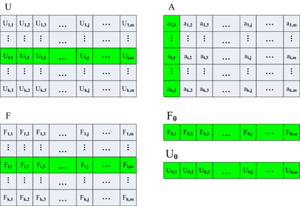
Figure 7.1 represents computational dependence for the elements
of matrix U(s+1) on (s+1)–th iterartion.
Figure 7.1 – Computational dependence for the elements
of matrix U(s+1)
The main feature of such way of calculations performing is necessity of recomputing of all k * m values of matrix
F(s). The given computing unit i contains only i-th line of matrix F(s).
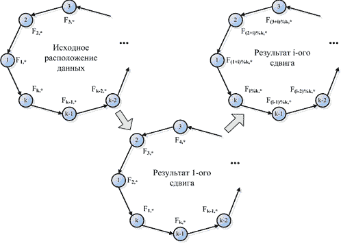
Let all processor units are incorporated according to their numbers in a ring (see figure 7.2). As it was been
described above, the unit i contains i-th row of matrix F(s). Elements of other rows can be obtained
via performing of their cyclic shift communication operation between processor units of a ring. Such shift operation
is performed (m–1) times on the step that is equal to 1. Each time after performing of such shift operation processor
units obtain the data that is required for algorithm computations. Different stages of cyclic shift operation are
presented in figure 7.2.
Figure 7.2 – Different stages of cyclic shift operation
ODE system solving time on all n to blocks without taking into account communication overhead is defined by the
formula (7.4). ODE function
 computation time is defined by
![Tf[delta]](../images/diss/temp7o7.gif) value, where
value, where
 is duration of the model time step (the designation is made in case of other sense of
 ). ).
 (7.4) (7.4)
Parallel algorithm acceleration of ODE system solving via single-step block method is defined by the formula (7.5)
(communication overhead is taken in account).
 (7.5) (7.5)
Figures 7.3 and 7.4 represent dependence of parallel algorithm acceleration on equations count and numbers block
points count correspondingly. There is no dependence of acceleration value on count of blocks.
Figure 7.3 – Dependence of parallel algorithm acceleration on ODE equations count (communication overhead is
taken in account)
Figure 7.4 – Dependence of parallel algorithm acceleration on block points count (communication overhead is
taken in account)
Efficiency of processor units utilizing by parallel algorithm is defined by the formula (7.6) (communication
overhead is taken in account).
 (7.6) (7.6)
Figures 7.5 and 7.6 represent dependence of parallel algorithm efficiency on equations count and numbers block
points count correspondingly. There is no dependence of efficiency value on count of blocks.
Figure 7.5 – Dependence of parallel algorithm efficiency on ODE equations count (communication overhead is taken
in account)
Figure 7.6 – Dependence of parallel algorithm efficiency on block points count (communication overhead is taken in
account)
|